TRamWAy - The Random Walk Analyzer - features tools for processing single-molecule localization microscopy data.
![]()
This notebook introduces the RWAnalyzer object and its main functionalities, as of version 0.5.
Table of contents
Let us first download the data required by this notebook:
from tutorial import *
download_RWAnalyzer_tour_data()
This notebook also requires some extra dependencies, including scikit-learn (required), stopit (optional) and those listed in the roi installation target for TRamWAy (only polytope is required).
import sys
!"{sys.executable}" -m pip install polytope cvxopt stopit scikit-learn
Requirement already satisfied: polytope in /home/francois/Projects/TRamWAy/lib/python3.8/site-packages (0.2.3) Requirement already satisfied: cvxopt in /home/francois/Projects/TRamWAy/lib/python3.8/site-packages (1.3.0) Requirement already satisfied: stopit in /home/francois/Projects/TRamWAy/lib/python3.8/site-packages (1.1.2) Requirement already satisfied: scikit-learn in /home/francois/Projects/TRamWAy/lib/python3.8/site-packages (1.2.2) Requirement already satisfied: scipy>=0.18.0 in /home/francois/Projects/TRamWAy/lib/python3.8/site-packages (from polytope) (1.10.1) Requirement already satisfied: numpy>=1.10.0 in /home/francois/Projects/TRamWAy/lib/python3.8/site-packages (from polytope) (1.24.2) Requirement already satisfied: networkx>=1.6 in /home/francois/Projects/TRamWAy/lib/python3.8/site-packages (from polytope) (3.0) Requirement already satisfied: threadpoolctl>=2.0.0 in /home/francois/Projects/TRamWAy/lib/python3.8/site-packages (from scikit-learn) (3.1.0) Requirement already satisfied: joblib>=1.1.1 in /home/francois/Projects/TRamWAy/lib/python3.8/site-packages (from scikit-learn) (1.2.0)
This notebook introduces (again) some basic concepts of the TRamWAy approach.
Some of the models inherited from InferenceMAP are used to estimate parameters of the dynamics of the fluorescent particles in the imaged biological sample. Such models focus on resolving the dynamics in space (and time), and are fed with individual displacements instead of entire trajectories.
Nevertheless, TRamWAy also features tools for extracting and quantifying trajectories, and two sections are dedicated to this topic.
Back to the mere TRamWAy approach that consists of resolving the dynamics in space, let us first have a look to example parameter maps.
Parameter maps
A key product TRamWAy generates out of single particle tracking data is a collection of parameter maps that quantify the local dynamics of the observed molecules and their environment.
Let us load a data file and visualize one such map before we dive into the details of getting these parameters:
from tramway.analyzer import *
a = RWAnalyzer()
a.spt_data.from_rwa_file('data-examples/demo1.rwa')
A .rwa file also stores the result of analyses on these data.
For example this file contains effective potential maps. Let us visualize them:
# retrieve parameter maps
sampling_label = 'gwr + 60s windowing'
sampling = a.spt_data.get_sampling(sampling_label)
map_label = 'dv d=50 v=2 (ns)'
maps = sampling.get_child(map_label)
# reload the time segmentation used to generate the maps
a.time.from_sampling(sampling)
%%capture
# initialize the movie for a parameter map
import matplotlib.pyplot as plt
fig, ax = plt.subplots(figsize=(8,7))
movie = a.mapper.mpl.animate(fig, maps, feature='potential',
axes=ax, unit='std', overlay_locations=True)
# render the movie
from IPython.display import HTML
HTML(movie.to_jshtml())
SPT analysis and data structures
Let us rewind and go step by step.
First, we initialized an RWAnalyzer object.
from tramway.analyzer import *
a = RWAnalyzer()
This object (here a) contains an attribute for addressing the single particle tracking data.
We initialized this attribute with a method that mutates the parent attribute itself and, in our case, loads a .rwa file:
a.spt_data.from_rwa_file('data-examples/demo1.rwa')
For coders who prefer explicit assignment, the following alternative syntax is allowed:
a.spt_data = spt_data.from_rwa_file('data-examples/demo1.rwa')
A .rwa file stores SPT data, together with results of the analyses performed on these data. The analysis results are organized in a tree:
from tutorial import *
print_analysis_tree(a.spt_data.analyses, annotations=True)
# `print(a.spt_data.analyses)` works similarly
<class 'pandas.core.frame.DataFrame'> <- original SPT data 'gwr + 60s windowing' <class 'tramway.tessellation.base.Partition'> <- data sampling 'dv d=50 v=2 (ns)' <class 'tramway.inference.base.Maps'> <- parameter maps
Here the tree features a single path, with the original data available at the top node:
a.spt_data.dataframe # or, equivalently, `a.spt_data.analyses.data`
| n | x | y | t | dx | dy | dt | |
|---|---|---|---|---|---|---|---|
| 0 | 3 | 41.0294 | 7.0758 | 20.48 | 0.0453 | 0.1043 | 0.04 |
| 1 | 4 | 41.0882 | 7.0933 | 30.16 | -0.0659 | 0.0746 | 0.04 |
| 2 | 5 | 41.0113 | 7.0608 | 30.36 | 0.0855 | 0.0980 | 0.04 |
| 3 | 6 | 41.0608 | 7.1048 | 30.60 | 0.0104 | 0.1294 | 0.04 |
| 4 | 7 | 41.0816 | 7.0902 | 30.68 | -0.0945 | 0.0432 | 0.04 |
| ... | ... | ... | ... | ... | ... | ... | ... |
| 12092 | 1856 | 41.0789 | 6.6456 | 794.88 | -0.0431 | 0.0354 | 0.04 |
| 12093 | 1856 | 41.0358 | 6.6810 | 794.92 | 0.0290 | -0.0924 | 0.04 |
| 12094 | 1856 | 41.0648 | 6.5886 | 794.96 | -0.0611 | 0.0485 | 0.04 |
| 12095 | 1856 | 41.0037 | 6.6371 | 795.00 | 0.0998 | -0.0704 | 0.04 |
| 12096 | 1856 | 41.1035 | 6.5667 | 795.04 | -0.0335 | 0.0785 | 0.04 |
12097 rows × 7 columns
The x and y columns represent space coordinates, t represents time, n is the trajectory index, and the other columns are displacement information that are not always present at this level.
The above analysis tree exhibits a single sampling of these data and a single set of parameter maps inferred from the so-sampled data. There could be multiple samplings of the initial trajectory data, and multiple sets of parameter maps for each sampling. A label helps identify each processing step.
In the RWAnalyzer object, in addition to the above dataframe, the spt_data attribute stores more information such as frame_interval and localization_error.
If this information was not automatically loaded from the file, we would set:
a.spt_data.frame_interval = 0.04 # in seconds
a.spt_data.localization_precision = 0.02 # in micrometers
The second level in the tree represents the data segmentation:
sampling_label = 'gwr + 60s windowing'
sampling = a.spt_data.get_sampling(sampling_label)
# `sampling.data` is `a.spt_data.analyses[sampling_label].data`
import matplotlib.pyplot as plt
fig, ax = plt.subplots(figsize=(7,7))
ax.set_title('molecule locations and partition')
a.tesseller.mpl.plot(sampling, axes=ax)

The above plot shows the location data and the spatial segmentation. In addition, the tessellation was combined with a time window, and the translocations were eventually assigned to the resulting spatio-temporal microdomains with extra constraints on the number of points per microdomain.
All this process is split in the tessellation, time segmentation and sampling of the data, and each step is controlled by a specific analyzer attribute.
The resulting data sampling found in the demo1.rwa file was obtained with the following parameters:
a.tesseller = tessellers.GWR
a.tesseller.resolution = .1
a.time.from_sliding_window(duration=60, shift=30)
a.sampler.from_nearest_neighbors(20)
The third level of the analysis tree stores maps of dynamics parameters resolved in space and time:
# retrieve parameter maps
map_label = 'dv d=50 v=2 (ns)'
maps = sampling.get_child(map_label)
# `maps.data` is `a.spt_data.analyses[sampling_label][map_label].data`
The above movie shows the time-varying diffusivity, which quantifies the random component in the local dynamics.
More inferred parameters are available in the maps object.
They are referred to as features, which names are explicitly listed in the object:
print(maps.data)
mode: stochastic.dv diffusivity_prior: 50 potential_prior: 2 jeffreys_prior: True runtime: 24088.606165647507 V0: 0 allow_negative_potential: True sigma: 0.02 stochastic: False features: ['diffusivity', 'potential', 'force'] maps: <class 'pandas.core.frame.DataFrame'>
As an example, we can generate a movie for another feature, say the effective potential:
%%capture
# initialize the movie for a parameter map
import matplotlib.pyplot as plt
fig, ax = plt.subplots(figsize=(8,7))
movie = a.mapper.mpl.animate(fig, maps, feature='diffusivity',
axes=ax, unit='std', overlay_locations=True, logscale=True)
# render the movie
from IPython.display import HTML
HTML(movie.to_jshtml())
These maps were obtained in a single inference with the following parameters:
a.mapper = models.DV()
a.mapper.diffusivity_prior = 50
a.mapper.potential_prior = 2
a.mapper.jeffreys_prior = True
a.mapper.V0 = 0 # flat initial potential
... and code:
def sample_and_infer(self):
""" `self` is the `RWAnalyzer` object """
for f in self.spt_data: # for each SPT data file (this also works with a single file)
# if not already loaded, the file is actually loaded at this point
sptdata = f.dataframe
# keep only the molecules that move by more than the localization error
sptdata = f.discard_static_trajectories(sptdata)
# apply the `tesseller.tessellate`, `time.segment` and `sampler.sample` steps all at once
sampling = self.sampler.sample(sptdata)
# parameter inference takes time...
maps = self.mapper.infer(sampling)
# wrap the original `sampling` and `maps` objects in node-like objects;
# this stores the analysis artefacts in the analysis tree for `f`
sampling = commit_as_analysis(sampling_label, sampling, parent=f)
maps = commit_as_analysis(map_label, maps, parent=sampling)
# save to file;
# in most cases, it is preferable to let the RWAnalyzer automatically determine the output filepath
f.analyses.save()
Here, sampler.sample calls the tessellate and segment methods of the tesseller and time attributes respectively. Of note, the sampler attribute would exhibit a working sample method even if not initialized.
At this point, sample_and_infer can run as-is:
sample_and_infer(a)
The code in the body of the function could run without making it a function,
but we do not want it to run now, as the infer step may take a few hours to complete.
As a function, the execution of sample_and_infer is also ready to be parallelized using the pipeline capability of RWAnalyzer.
For example, with a few additional lines of code, sample_and_infer execution can be delegated to a computer cluster and the resulting output file(s) retrieved onto the host that runs the Jupyter notebook.
Summary
Before any analysis is run and an output .rwa file is generated, the SPT data often come as a text file.
To sum up, and as a transition to the next section, let us export the SPT data to an ascii file and start from scratch without printing or plotting anything:
a.spt_data.to_ascii_file('data-examples/demo1.txt')
from tramway.analyzer import *
a = RWAnalyzer()
Note the main difference:
a.spt_data.from_ascii_file('data-examples/demo1.txt')
a.spt_data.frame_interval = 0.04 # in seconds
a.spt_data.localization_precision = 0.02 # in micrometers
a.tesseller = tessellers.GWR
a.tesseller.resolution = .1
a.time.from_sliding_window(duration=60, shift=30)
a.sampler.from_nearest_neighbors(20)
a.mapper = models.DV()
a.mapper.diffusivity_prior = 50
a.mapper.potential_prior = 2
a.mapper.jeffreys_prior = True
a.mapper.V0 = 0 # flat initial potential
... and we are ready!
# sample_and_infer(a)
Note that, if you want to adapt sampling_label and map_label, you will have to redefine sample_and_infer.
Locations, trajectories and translocations
Location and displacement information is made available in pandas.DataFrames. However, there are subtle differences between trajectories and translocations.
Let us load some localization data:
import pandas as pd
pd.set_option('display.max_rows', 8)
from tramway.core import load_xyt
locations = load_xyt('data-examples/c05_low_density.tsf.xyt', columns=list('xyt'))
locations
| x | y | t | |
|---|---|---|---|
| 0 | 26.6615 | 39.5796 | 0.06 |
| 1 | 26.1820 | 43.4160 | 0.06 |
| 2 | 27.0411 | 26.9305 | 0.06 |
| 3 | 29.1381 | 48.5524 | 0.06 |
| ... | ... | ... | ... |
| 33547 | 55.8001 | 45.0347 | 31.20 |
| 33548 | 59.9244 | 36.4617 | 31.20 |
| 33549 | 58.5234 | 29.2296 | 31.20 |
| 33550 | 58.7866 | 36.8735 | 31.20 |
33551 rows × 3 columns
The x and y columns represent space, in $\mu m$, and t represents time, in $s$.
The frame interval appears to be 0.06 and, as can be seen above in the dataframe, the locations are ordered in time.
The tramway.core module exports convenience functions like iter_frames to loop over the locations grouped by frame.
Localization data tracking
Let us track these data using the non-tracking tracker:
from tramway.analyzer import *
a = RWAnalyzer()
a.tracker.from_non_tracking()
a.tracker.frame_interval = 0.06
This algorithm requires some hint about the values expected for diffusivity, plus an indication about the localization precision or error:
a.tracker.estimated_high_diffusivity = 0.3
a.tracker.localization_precision = 0.03
Side note
Some key parameters such as frame_interval and localization_precision are available at multiple places.
These parameters are actually stored in the spt_data attribute:
a.spt_data.frame_interval
0.06
This has been made possible by the tracker attribute altering the spt_data attribute:
a.spt_data
<tramway.analyzer.spt_data.TrackerOutput at 0x7f1de0866a40>
... while it was beforehands:
RWAnalyzer().spt_data
<tramway.analyzer.spt_data.SPTDataInitializer at 0x7f1de076e180>
Tracking (continued)
a.tracker.track(locations, register=True)
| n | x | y | t | |
|---|---|---|---|---|
| 0 | 1 | 26.1820 | 43.4160 | 0.06 |
| 1 | 1 | 26.2917 | 43.2076 | 0.12 |
| 2 | 2 | 27.0411 | 26.9305 | 0.06 |
| 3 | 2 | 27.3263 | 26.7477 | 0.12 |
| ... | ... | ... | ... | ... |
| 12851 | 5098 | 47.0593 | 36.7691 | 31.14 |
| 12852 | 5098 | 47.3644 | 36.9945 | 31.20 |
| 12853 | 5099 | 36.9425 | 36.9245 | 31.14 |
| 12854 | 5099 | 36.7721 | 37.0181 | 31.20 |
12855 rows × 4 columns
The track method applied to the example localization file returned a pandas.DataFrame that represents the resulting trajectories.
Column n encodes the trajectory index.
Rows are locations, ordered first by trajectory index and second by time.
The register=True option made track append the series of trajectories to the spt_data attribute:
for f in a.spt_data:
pass
f.dataframe
| n | x | y | t | |
|---|---|---|---|---|
| 0 | 1 | 26.1820 | 43.4160 | 0.06 |
| 1 | 1 | 26.2917 | 43.2076 | 0.12 |
| 2 | 2 | 27.0411 | 26.9305 | 0.06 |
| 3 | 2 | 27.3263 | 26.7477 | 0.12 |
| ... | ... | ... | ... | ... |
| 12851 | 5098 | 47.0593 | 36.7691 | 31.14 |
| 12852 | 5098 | 47.3644 | 36.9945 | 31.20 |
| 12853 | 5099 | 36.9425 | 36.9245 | 31.14 |
| 12854 | 5099 | 36.7721 | 37.0181 | 31.20 |
12855 rows × 4 columns
Note here that we had to loop over items in a.spt_data.
Indeed, the track method can be called multiple times, on different files, and consequently the spt_data attribute could contain multiple items.
Because these data provider attributes (others are images and roi) are always iterable and often contain a single item, the tramway.analyzer package exports some very simple convenience functions to get the first or unique item of such iterators:
trajectories = single(a.spt_data).dataframe
trajectories
| n | x | y | t | |
|---|---|---|---|---|
| 0 | 1 | 26.1820 | 43.4160 | 0.06 |
| 1 | 1 | 26.2917 | 43.2076 | 0.12 |
| 2 | 2 | 27.0411 | 26.9305 | 0.06 |
| 3 | 2 | 27.3263 | 26.7477 | 0.12 |
| ... | ... | ... | ... | ... |
| 12851 | 5098 | 47.0593 | 36.7691 | 31.14 |
| 12852 | 5098 | 47.3644 | 36.9945 | 31.20 |
| 12853 | 5099 | 36.9425 | 36.9245 | 31.14 |
| 12854 | 5099 | 36.7721 | 37.0181 | 31.20 |
12855 rows × 4 columns
We can now run the same type of analyses on the SPT data, as presented before.
Representations for trajectories and translocations
The models underlying the main inference methods available in TRamWAy do not need entire trajectories, but only individual displacements, or translocations.
To make the notion of translocation visible, let us define a region of interest and crop the data within this ROI:
a.spt_data.bounds
| n | x | y | t | |
|---|---|---|---|---|
| min | 1.0 | 19.8098 | 19.2550 | 0.06 |
| max | 5099.0 | 61.5214 | 58.6531 | 31.20 |
from tramway.core import crop
cropped_trajectories = crop(trajectories, [20.,20.,10.,10.], keep_nan=True)
cropped_trajectories
| n | x | y | t | dx | dy | dt | |
|---|---|---|---|---|---|---|---|
| 0 | 3 | 27.0411 | 26.9305 | 0.06 | 0.2852 | -0.1828 | 0.06 |
| 1 | 3 | 27.3263 | 26.7477 | 0.12 | NaN | NaN | NaN |
| 2 | 4 | 27.2278 | 26.7087 | 0.24 | 0.1957 | -0.1466 | 0.06 |
| 3 | 4 | 27.4235 | 26.5621 | 0.30 | NaN | NaN | NaN |
| ... | ... | ... | ... | ... | ... | ... | ... |
| 95 | 47 | 27.0603 | 28.2362 | 29.34 | -0.0411 | 0.2687 | 0.06 |
| 96 | 47 | 27.0192 | 28.5049 | 29.40 | NaN | NaN | NaN |
| 97 | 48 | 22.5607 | 28.6995 | 30.12 | 0.0184 | 0.0718 | 0.06 |
| 98 | 48 | 22.5791 | 28.7713 | 30.18 | NaN | NaN | NaN |
99 rows × 7 columns
We took a (huge) 10x10$\mu m$ area and found a hundred locations in it (these data are indeed low-density, as the filename stated).
delta columns were added: dx, dy and dt.
They encode the displacement from the location described in the same row.
The terminal location for each trajectory exhibits undefined delta values (NaN). As such, the above data are still considered as trajectory data.
Translocations are the rows with defined displacement information:
translocations = crop(trajectories, [20.,20.,10.,10.])
translocations
| n | x | y | t | dx | dy | dt | |
|---|---|---|---|---|---|---|---|
| 0 | 3 | 27.0411 | 26.9305 | 0.06 | 0.2852 | -0.1828 | 0.06 |
| 1 | 4 | 27.2278 | 26.7087 | 0.24 | 0.1957 | -0.1466 | 0.06 |
| 2 | 6 | 25.1349 | 23.8702 | 1.56 | 0.1845 | 0.0494 | 0.06 |
| 3 | 7 | 24.7621 | 27.4019 | 1.62 | -0.1749 | 0.1544 | 0.06 |
| ... | ... | ... | ... | ... | ... | ... | ... |
| 49 | 46 | 24.5129 | 25.5778 | 28.56 | -0.0652 | -0.0410 | 0.06 |
| 50 | 46 | 24.4477 | 25.5368 | 28.62 | 0.1256 | 0.0381 | 0.06 |
| 51 | 47 | 27.0603 | 28.2362 | 29.34 | -0.0411 | 0.2687 | 0.06 |
| 52 | 48 | 22.5607 | 28.6995 | 30.12 | 0.0184 | 0.0718 | 0.06 |
53 rows × 7 columns
Some methods, e.g. for plotting trajectories, explicitly require trajectory data, while other methods require translocations only.
The tramway.core package exports conversion functions such as trajectories_to_translocations and translocations_to_trajectories.
This package also exports the iter_frames and iter_trajectories functions to iterate such dataframes over groups of rows.
ROI definition
The above cropping can be generalized to many regions of interest using the roi attribute.
Regions of interest can be defined in many ways, as square areas centered at e.g. density peaks, or bounding boxes on the coordinates, including time, etc.
from tramway.analyzer import *
a = RWAnalyzer()
a.tracker.from_non_tracking()
a.tracker.frame_interval = 0.06
a.tracker.estimated_high_diffusivity = 0.3
a.tracker.localization_precision = 0.03
from tramway.core import load_xyt
for source in (
'data-examples/Manip01-01-Beta400AA-01-15ms.rpt.xyt',
'data-examples/Manip01-01-Beta400AA-02-15ms.rpt.xyt'):
xyt = load_xyt(source, columns=['x', 'y', 'frame index'])
xyt['t'] = xyt['frame index'] * a.tracker.frame_interval
a.tracker.track(xyt, source=source, register=True)
from tramway.analyzer.roi.utils import *
import matplotlib.pyplot as plt
roi_size = 1.
_, axes = plt.subplots(1, len(a.spt_data), figsize=(16,8))
for f, ax in zip(a.spt_data, axes):
# identify density peaks
roi_centers = density_based_roi(f.dataframe, .0075)
# define square ROI centered on the peaks
f.roi.from_squares(roi_centers, roi_size)
# plot the data
f.mpl.plot(axes=ax)

As of version 0.5, the encouraged way to store such ROI center or boundary information is additional text files similar to SPT ascii files, with similar filenames as well, using a suffix before the extension to differenciate between SPT and ROI files.
import numpy as np
import pandas as pd
import os
for f in a.spt_data:
basename, _ = os.path.splitext(f.source)
# in this example, because column 'frame index' has a space in its name,
# we should either rename it (e.g. as 'frame_index') or skip it as below:
f.to_ascii_file(basename+'.txt', columns=['n', 'x', 'y', 't'])
f.roi.to_ascii_file(basename+'-roi.txt')
Let us simply print the number of translocations per ROI:
a = RWAnalyzer()
a.spt_data.from_ascii_files('data-examples/Manip01-01-Beta400AA-*-15ms.rpt.txt')
a.roi.from_ascii_files(suffix='-roi') # '-roi' is the default suffix and can be omitted
for r in a.roi.as_support_regions():
# get the translocations that originate from within the roi bounding box
sptdata = r.crop()
# the `source` attribute points to the spt data source;
# the `label` attribute is the default label for any sampling of the ROI data
print(r.source, r.label, len(sptdata), sep='\t')
data-examples/Manip01-01-Beta400AA-01-15ms.rpt.txt roi000 464 data-examples/Manip01-01-Beta400AA-01-15ms.rpt.txt roi001 671 data-examples/Manip01-01-Beta400AA-01-15ms.rpt.txt roi002 817 data-examples/Manip01-01-Beta400AA-01-15ms.rpt.txt roi003 612 data-examples/Manip01-01-Beta400AA-01-15ms.rpt.txt roi004 457 data-examples/Manip01-01-Beta400AA-01-15ms.rpt.txt roi005 868 data-examples/Manip01-01-Beta400AA-01-15ms.rpt.txt roi006 727 data-examples/Manip01-01-Beta400AA-01-15ms.rpt.txt roi007 3513 data-examples/Manip01-01-Beta400AA-01-15ms.rpt.txt roi008 902 data-examples/Manip01-01-Beta400AA-01-15ms.rpt.txt roi009 764 data-examples/Manip01-01-Beta400AA-01-15ms.rpt.txt roi010 1004 data-examples/Manip01-01-Beta400AA-01-15ms.rpt.txt roi011 884 data-examples/Manip01-01-Beta400AA-01-15ms.rpt.txt roi012 701 data-examples/Manip01-01-Beta400AA-01-15ms.rpt.txt roi013 957 data-examples/Manip01-01-Beta400AA-01-15ms.rpt.txt roi014 1041 data-examples/Manip01-01-Beta400AA-01-15ms.rpt.txt roi015 902 data-examples/Manip01-01-Beta400AA-01-15ms.rpt.txt roi016 822 data-examples/Manip01-01-Beta400AA-01-15ms.rpt.txt roi017 589 data-examples/Manip01-01-Beta400AA-01-15ms.rpt.txt roi018 382 data-examples/Manip01-01-Beta400AA-01-15ms.rpt.txt roi019 826 data-examples/Manip01-01-Beta400AA-01-15ms.rpt.txt roi020 664 data-examples/Manip01-01-Beta400AA-01-15ms.rpt.txt roi021 705 data-examples/Manip01-01-Beta400AA-02-15ms.rpt.txt roi000 250 data-examples/Manip01-01-Beta400AA-02-15ms.rpt.txt roi001 257 data-examples/Manip01-01-Beta400AA-02-15ms.rpt.txt roi002 186 data-examples/Manip01-01-Beta400AA-02-15ms.rpt.txt roi003 327 data-examples/Manip01-01-Beta400AA-02-15ms.rpt.txt roi004 406 data-examples/Manip01-01-Beta400AA-02-15ms.rpt.txt roi005 334 data-examples/Manip01-01-Beta400AA-02-15ms.rpt.txt roi006 278 data-examples/Manip01-01-Beta400AA-02-15ms.rpt.txt roi007 323 data-examples/Manip01-01-Beta400AA-02-15ms.rpt.txt roi008 488 data-examples/Manip01-01-Beta400AA-02-15ms.rpt.txt roi009 321 data-examples/Manip01-01-Beta400AA-02-15ms.rpt.txt roi010 524 data-examples/Manip01-01-Beta400AA-02-15ms.rpt.txt roi011 393 data-examples/Manip01-01-Beta400AA-02-15ms.rpt.txt roi012 396 data-examples/Manip01-01-Beta400AA-02-15ms.rpt.txt roi013 280 data-examples/Manip01-01-Beta400AA-02-15ms.rpt.txt roi014 228 data-examples/Manip01-01-Beta400AA-02-15ms.rpt.txt roi015 253 data-examples/Manip01-01-Beta400AA-02-15ms.rpt.txt roi016 322 data-examples/Manip01-01-Beta400AA-02-15ms.rpt.txt roi017 212 data-examples/Manip01-01-Beta400AA-02-15ms.rpt.txt roi018 441 data-examples/Manip01-01-Beta400AA-02-15ms.rpt.txt roi019 381 data-examples/Manip01-01-Beta400AA-02-15ms.rpt.txt roi020 452 data-examples/Manip01-01-Beta400AA-02-15ms.rpt.txt roi021 188 data-examples/Manip01-01-Beta400AA-02-15ms.rpt.txt roi022 198 data-examples/Manip01-01-Beta400AA-02-15ms.rpt.txt roi023 217 data-examples/Manip01-01-Beta400AA-02-15ms.rpt.txt roi024 180 data-examples/Manip01-01-Beta400AA-02-15ms.rpt.txt roi025 185 data-examples/Manip01-01-Beta400AA-02-15ms.rpt.txt roi026 249 data-examples/Manip01-01-Beta400AA-02-15ms.rpt.txt roi027 214 data-examples/Manip01-01-Beta400AA-02-15ms.rpt.txt roi028 242 data-examples/Manip01-01-Beta400AA-02-15ms.rpt.txt roi029 208 data-examples/Manip01-01-Beta400AA-02-15ms.rpt.txt roi030 272 data-examples/Manip01-01-Beta400AA-02-15ms.rpt.txt roi031 290 data-examples/Manip01-01-Beta400AA-02-15ms.rpt.txt roi032 212 data-examples/Manip01-01-Beta400AA-02-15ms.rpt.txt roi033 185 data-examples/Manip01-01-Beta400AA-02-15ms.rpt.txt roi034 154 data-examples/Manip01-01-Beta400AA-02-15ms.rpt.txt roi035 160 data-examples/Manip01-01-Beta400AA-02-15ms.rpt.txt roi036 169 data-examples/Manip01-01-Beta400AA-02-15ms.rpt.txt roi037 204 data-examples/Manip01-01-Beta400AA-02-15ms.rpt.txt roi038 252 data-examples/Manip01-01-Beta400AA-02-15ms.rpt.txt roi039 210 data-examples/Manip01-01-Beta400AA-02-15ms.rpt.txt roi040 217 data-examples/Manip01-01-Beta400AA-02-15ms.rpt.txt roi041 367 data-examples/Manip01-01-Beta400AA-02-15ms.rpt.txt roi042 270 data-examples/Manip01-01-Beta400AA-02-15ms.rpt.txt roi043 367 data-examples/Manip01-01-Beta400AA-02-15ms.rpt.txt roi044 228 data-examples/Manip01-01-Beta400AA-02-15ms.rpt.txt roi045 229 data-examples/Manip01-01-Beta400AA-02-15ms.rpt.txt roi046 300 data-examples/Manip01-01-Beta400AA-02-15ms.rpt.txt roi047 248 data-examples/Manip01-01-Beta400AA-02-15ms.rpt.txt roi048 226 data-examples/Manip01-01-Beta400AA-02-15ms.rpt.txt roi049 545 data-examples/Manip01-01-Beta400AA-02-15ms.rpt.txt roi050 315 data-examples/Manip01-01-Beta400AA-02-15ms.rpt.txt roi051 234 data-examples/Manip01-01-Beta400AA-02-15ms.rpt.txt roi052 162 data-examples/Manip01-01-Beta400AA-02-15ms.rpt.txt roi053 341 data-examples/Manip01-01-Beta400AA-02-15ms.rpt.txt roi054 299 data-examples/Manip01-01-Beta400AA-02-15ms.rpt.txt roi055 248 data-examples/Manip01-01-Beta400AA-02-15ms.rpt.txt roi056 146 data-examples/Manip01-01-Beta400AA-02-15ms.rpt.txt roi057 187 data-examples/Manip01-01-Beta400AA-02-15ms.rpt.txt roi058 335 data-examples/Manip01-01-Beta400AA-02-15ms.rpt.txt roi059 326 data-examples/Manip01-01-Beta400AA-02-15ms.rpt.txt roi060 355 data-examples/Manip01-01-Beta400AA-02-15ms.rpt.txt roi061 312 data-examples/Manip01-01-Beta400AA-02-15ms.rpt.txt roi062 374 data-examples/Manip01-01-Beta400AA-02-15ms.rpt.txt roi063 370 data-examples/Manip01-01-Beta400AA-02-15ms.rpt.txt roi064 365 data-examples/Manip01-01-Beta400AA-02-15ms.rpt.txt roi065 309 data-examples/Manip01-01-Beta400AA-02-15ms.rpt.txt roi066 286 data-examples/Manip01-01-Beta400AA-02-15ms.rpt.txt roi067 190 data-examples/Manip01-01-Beta400AA-02-15ms.rpt.txt roi068 199 data-examples/Manip01-01-Beta400AA-02-15ms.rpt.txt roi069 339 data-examples/Manip01-01-Beta400AA-02-15ms.rpt.txt roi070 369 data-examples/Manip01-01-Beta400AA-02-15ms.rpt.txt roi071 229 data-examples/Manip01-01-Beta400AA-02-15ms.rpt.txt roi072 281 data-examples/Manip01-01-Beta400AA-02-15ms.rpt.txt roi073 277 data-examples/Manip01-01-Beta400AA-02-15ms.rpt.txt roi074 268 data-examples/Manip01-01-Beta400AA-02-15ms.rpt.txt roi075 218 data-examples/Manip01-01-Beta400AA-02-15ms.rpt.txt roi076 235 data-examples/Manip01-01-Beta400AA-02-15ms.rpt.txt roi077 708 data-examples/Manip01-01-Beta400AA-02-15ms.rpt.txt roi078 206 data-examples/Manip01-01-Beta400AA-02-15ms.rpt.txt roi079 208 data-examples/Manip01-01-Beta400AA-02-15ms.rpt.txt roi080 181 data-examples/Manip01-01-Beta400AA-02-15ms.rpt.txt roi081 252 data-examples/Manip01-01-Beta400AA-02-15ms.rpt.txt roi082 239
Strategies for overlapping ROI
Regions of interest may exhibit some overlap, which is to be expected when they are automatically identified. In the case of overlapping ROI, it usually makes sense to group these regions before segmenting the data and inferring model parameters.
Initializer methods for the roi attribute feature an optional group_overlapping_roi argument that can be set to True.
This combines the input ROI into so-called support regions for data processing, while the original ROI, termed individual roi, operate as windows on the corresponding support region.
a = RWAnalyzer()
a.spt_data.from_ascii_files('data-examples/Manip01-01-Beta400AA-*-15ms.rpt.txt')
a.roi.from_ascii_files(suffix='roi', group_overlapping_roi=True)
_, axes = plt.subplots(1, len(a.spt_data), figsize=(16,8))
for f, ax in zip(a.spt_data, axes):
f.mpl.plot(axes=ax, sup_color='blue')

In the above figures, the blue rectangles depict the rectangular bounding box of support regions, whereas support regions are not necessarily rectangles. Indeed, a support region is a union of ROI, no more.
As a consequence, the roi attribute can be iterated in two ways.
One can loop over either the individual ROI or the support regions, with the as_individual_roi or as_support_regions methods respectively.
Choosing what to iterate is made a requirement, and the roi attribute itself cannot be iterated as is.
Even if no grouping is performed (default behavior), as_support_regions should be used instead of as_individual_roi for data processing, including segmentation and standard inference,
especially as as_individual_roi is not supported yet by some flavors of parallel processing, and an exception may be raised at the time of dispatching tasks with ROI granularity.
For post-mapping analysis, the support regions can be accessed from the individual ROI, but only when as_individual_roi is called from an SPT data item (f.roi and not a.roi):
n = 0
for f in a.spt_data:
for roi_index, roi_obj in f.roi.as_individual_roi(return_index=True):
if 20 < n:
break
n += 1
support_region = f.roi.get_support_region(roi_index)
print(f'{roi_obj.label} lies in support region:\t{support_region.label}')
print('...')
roi000 lies in support region: roi000 roi001 lies in support region: roi001 roi002 lies in support region: roi002-003 roi003 lies in support region: roi002-003 roi004 lies in support region: roi004-005 roi005 lies in support region: roi004-005 roi006 lies in support region: roi006 roi007 lies in support region: roi007 roi008 lies in support region: roi008-009-010-011 roi009 lies in support region: roi008-009-010-011 roi010 lies in support region: roi008-009-010-011 roi011 lies in support region: roi008-009-010-011 roi012 lies in support region: roi012-014-015 roi013 lies in support region: roi013 roi014 lies in support region: roi012-014-015 roi015 lies in support region: roi012-014-015 roi016 lies in support region: roi016-019 roi017 lies in support region: roi017 roi018 lies in support region: roi018 roi019 lies in support region: roi016-019 roi020 lies in support region: roi020 ...
The connection between a ROI and the corresponding support region is not made easier than demonstrated above, because ROI can also be defined in multiple collections, with different labels (instead of the simple 'roi' label), possibly corresponding to different experimental conditions to be compared, while still having support regions that can group ROI from different collections.
Tessellation
To resolve the dynamics in space, TRamWAy offers several approaches for segmenting the space. These segmentation approaches all consist of partitioning the space into cells. They offer a basis for sampling the data into microdomains that may overlap as explained in the sampling section.
One of the most basic spatial segmentation approaches draws hexagonal tiles:
from tramway.analyzer import *
import matplotlib.pyplot as plt
a = RWAnalyzer()
a.spt_data.from_ascii_file('data-examples/demo1.txt')
a.spt_data.localization_precision = 0.02
a.spt_data.frame_interval = 0.04
a.tesseller = tessellers.Hexagons
as_ = a.sampler.sample(a.spt_data.dataframe)
fig, ax = plt.subplots(1,1, figsize=(7.2,8))
a.tesseller.mpl.plot(as_, axes=ax, title='regular mesh with hexagonal tiles')

Another method, that adapts to the local density or local displacement length, is based on the Growing-When-Required self-organizing graph technique:
b = RWAnalyzer()
b.tesseller = tessellers.GWR
b.tesseller.topology = 'approximate density'
b.tesseller.resolution = 0.1
c = RWAnalyzer()
c.tesseller = tessellers.GWR
c.tesseller.topology = 'displacement length'
c.tesseller.resolution = 0.1
np.random.seed(23794837)
bs = b.sampler.sample(a.spt_data.dataframe)
np.random.seed(23794837)
cs = c.sampler.sample(a.spt_data.dataframe)
_, ax = plt.subplots(1,2, figsize=(16,8))
b.tesseller.mpl.plot(bs, axes=ax[0], title='adaptive mesh driven by local density')
c.tesseller.mpl.plot(cs, axes=ax[1], title='adaptive mesh driven by local displacement length')
/home/francois/Projects/TRamWAy/tramway/tessellation/gwr/gas.py:313: RuntimeWarning: Rounding error: negative distance
warnings.warn("Rounding error: negative distance", RuntimeWarning)

Each tessellation approach offers specific parameters in addition to the general resolution parameter that is differently interpreted by the different approaches.
Most methods are referenced in the documentation and RWAnalyzer-adapted wrappers are featured by the tessellers module object for some of the available methods.
Side effects
Note that we initialized multiple RWAnalyzer objects to process the data from only one analyzer object.
Generally this is not recommended. The attributes that represent specific processing steps may access other attributes to gather all the necessary information. As a consequence, side effects are to be expected.
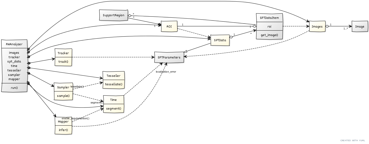
Almost all the attributes access general parameters such as frame_interval and localization_error that are stored in the spt_data attribute.
Other dependencies exist in the sampler attribute that accesses the tesseller and time attributes, and in the mapper attribute that also accesses the time attribute.
More about side effects
To prevent reusing analyzer objects, which may cause side effects, assigning a new value to an initialized attribute is not allowed:
%%script python3 --no-raise-error
from tramway.analyzer import *
a = RWAnalyzer()
a.spt_data = spt_data.from_ascii_file('data-examples/demo1.txt')
df = a.spt_data.dataframe
# not allowed!
a.spt_data = spt_data.from_dataframe(df)
Traceback (most recent call last): File "<stdin>", line 2, in <module> ModuleNotFoundError: No module named 'tramway'
To allow attribute overwrite, and show an example side effect:
import warnings
warnings.simplefilter('ignore', SideEffectWarning)
a = RWAnalyzer()
a.spt_data = spt_data.from_ascii_file('data-examples/demo1.txt')
a.spt_data.localization_precision = 0.03
a.time.frame_interval = 0.05 # this actually sets `frame_interval` in `spt_data`
former_spt_data = a.spt_data
a.spt_data = spt_data.from_dataframe(former_spt_data.dataframe)
a.spt_data.localization_error = former_spt_data.localization_error
a.spt_data.dt = former_spt_data.dt # `dt` is an alias for `frame_interval`
dict(
localization_precision = a.spt_data.localization_precision,
frame_interval = a.spt_data.frame_interval )
{'localization_precision': 0.03, 'frame_interval': 0.05}
Some overwritting use cases are allowed through specific methods such as reload_from_rwa_files that can be called when SPT data are processed from ascii files on a remote host, and retrieved as .rwa files onto the local host, to reload the resulting analysis trees from these .rwa files corresponding to the input ascii files.
Other methods
Some tessellation methods such as InferenceMAP's quadtree, called kdtree in TRamWAy, are not available as dedicated wrappers. They can be loaded as plugins:
d = RWAnalyzer()
d.tesseller.from_plugin('kdtree')
d.tesseller.resolution = 0.05
ds = d.sampler.sample(a.spt_data.dataframe)
_, ax = plt.subplots(1,1, figsize=(7.2,8))
d.tesseller.mpl.plot(ds, axes=ax, title='quad-tree')

Time segmentation
In addition to tessellating the space, the data can also be segmented into time segments, often using a sliding window:
from tramway.analyzer import *
import matplotlib.pyplot as plt
a = RWAnalyzer()
a.spt_data.from_ascii_file('data-examples/demo1.txt')
a.spt_data.localization_precision = 0.02
a.spt_data.frame_interval = 0.04
a.tesseller = tessellers.Hexagons
a.time.from_sliding_window(60) # window duration in seconds
a.time.window_shift = 45 # in seconds; this introduces a 25%-overlap between successive segments (default is no overlap)
sampling = a.sampler.sample(a.spt_data.dataframe)
One can iterate over the resulting time segments, as the following example that prints the number of translocations assigned to each segment:
for times, individual_segment_sampling in a.time.as_time_segments(sampling, return_times=True):
print(
a.time.segment_label(None, times, sampling),
len(individual_segment_sampling.points),
sep=': \t',
)
t=20.48-80.48s: 186 t=65.48-125.48s: 730 t=110.48-170.48s: 1048 t=155.48-215.48s: 1339 t=200.48-260.48s: 1365 t=245.48-305.48s: 1142 t=290.48-350.48s: 933 t=335.48-395.48s: 981 t=380.48-440.48s: 750 t=425.48-485.48s: 526 t=470.48-530.48s: 826 t=515.48-575.48s: 1250 t=560.48-620.48s: 1119 t=605.48-665.48s: 1100 t=650.48-710.48s: 964 t=695.48-755.48s: 975 t=740.48-800.48s: 925
A movie can be generated to visualize these points:
%%capture
fig, _ = plt.subplots(figsize=(7,7))
movie = a.tesseller.mpl.animate(fig, sampling)
from IPython.display import HTML
HTML(movie.to_jshtml())
Sampling
More importantly, these spatial and temporal segmentations are used to sample the (trans-)location data. The default approach -- e.g. for space -- consists of partitioning, i.e. assigning to each microdomain all the points that lie within the corresponding Voronoi cell. The Voronoi cells are illustrated as meshes in red in previous figures and movies.
However, the segmentations actually define the microdomains as center points only. The extent of the microdomains may be overriden so that a given point can be assigned to multiple microdomains, or none.
Data sampling is controlled by the sampler attribute.
It features several initializers, including from_voronoi (default behavior), from_spheres and from_nearest_neighbors that implement different behaviors along the spatial dimensions, and from_nearest_time_neighbors for adapting the time window locally.
All the samplers first operate like from_voronoi and then perform local adjustments so as to enforce criteria such as a lower bound on the number of assigned points per microdomain.
Using alternative samplers, it is actually possible to assign data to microdomains that originally (following the default/initial behavior) do not contain any point.
This can also be controlled with an attribute common to all the samplers: min_location_count.
In the former API (the tessellate function), this parameter is 1 per default, while it is 0 here.
The resulting segmentations are better illustrated with a color map and, as a consequence, an example sampling is explained in further details in the next section.
Parameter estimation
Once microdomains are defined, with their respective (trans-)location data, all sorts of estimates can be extracted in each microdomain, taken individually or altogether, using the mapper attribute of an RWAnalyzer object.
TRamWAy features several inference procedures for models borrowed from InferenceMAP.
DV inference
As showed in previous sections, the DV model explains the observed displacements as resulting from a diffusive term and a drift component derived from a potential lanscape:
$\frac{d\textbf{r}}{dt} = \sqrt{2D(\textbf{r})} \xi(t) - D(\textbf{r}) \frac{\nabla V(\textbf{r})}{k_{\textrm{B}}T}$
This model jointly estimates the local diffusivities $D$ (in $\mu m^2. s^{-1}$ if coordinates $\textbf{r}$ are expressed as $\mu m$) and effective potentials $V$ (expressed as $k_{\textrm{B}}T$), and can be defined and applied in different ways:
- the 'dv' plugin, or equivalently
models.DV('original'), suitable for moderate numbers of microdomains and, if a sliding window is applied to segment the data, as long as no time regularization is performed - the 'stochastic.dv' plugin, or equivalently
models.DV('stochastic'), suitable for large inferences (many microdomains) and time-regularized inferences - the 'semi.stochastic.dv' plugin, or equivalently
models.DV(start='stochastic'), that comes as an improvement ofmodels.DV('stochastic')for moderately large inference, with additional non-stochastic fine-tuning iterations after a first stochastic convergence phase
All these variants can be interrupted. In addition, 'stochastic.dv' admits a timeout, which makes it a better candidate for a rapid demonstration. Let us go straight to the figures, and then explain.
Define the processing steps
from tramway.analyzer import *
import matplotlib.pyplot as plt
a = RWAnalyzer()
a.spt_data.from_ascii_file('data-examples/demo1.txt')
a.spt_data.localization_precision = 0.02
a.tesseller = tessellers.Hexagons
a.sampler.from_nearest_neighbors(10)
a.sampler.min_location_count = 1
a.mapper = models.DV('stochastic')
a.mapper.diffusivity_prior = 20
a.mapper.potential_prior = 1
a.mapper.max_runtime = 10 # in seconds; note that if TRamWAy does not find the stopit package, this argument is ignored and the inference takes about 10 minutes
a.mapper.verbose = True
Process
# step 1. read the data
translocation_data = a.spt_data.dataframe
# step 2. sample the data
data_sampling = a.sampler.sample(translocation_data)
# step 3. estimate the model parameters
inferred_parameters = a.mapper.infer(data_sampling)
number of workers: 15
At iterate 12 f(102)= -1.209999E+03 df= -1.694982E+00 proj g = 1.205690E+00
At iterate 5 f(54)= -5.307699E+02 df= -3.080154E-01 proj g = 1.121731E+00
At iterate 10 f(109)= -2.142904E+03 df= -7.262673E+00 proj g = 2.292387E+01
At iterate 7 f(75)= -3.229529E+02 df= -1.563738E-01 proj g = 2.040201E-01
At iterate 15 f(38)= -4.385403E+03 df= -5.803366E+00 proj g = 1.282256E+01
At iterate 4 f(68)= -1.527292E+03 df= -5.469015E-01 proj g = 9.276491E-01
At iterate 1 f(31)= -3.266136E+03 df= -4.695156E+00 proj g = 6.958643E+00
At iterate 8 f(104)= -7.483543E+02 df= -4.440981E-01 proj g = 3.126877E-01
At iterate 16 f( 5)= -2.475111E+02 df= -4.712139E-01 proj g = 8.854475E-01
At iterate 13 f(9)= -2.651737E+02 df= -2.546332E-01 proj g = 2.141034E-01
At iterate 3 f(35)= -5.788881E+02 df= -1.423732E+00 proj g = 7.716343E-01
At iterate 6 f(80)= -3.408521E+03 df= -4.668102E+00 proj g = 1.187236E+01
At iterate 2 f(25)= -6.265032E+02 df= -2.679749E+00 proj g = 1.382210E+00
At iterate 14 f(14)= -5.789424E+02 df= -1.186109E+00 proj g = 8.684016E-01
At iterate 11 f(29)= -3.331172E+03 df= -1.778256E+00 proj g = 1.875073E+00
At iterate 9 f(105)= -6.937148E+02 df= -2.508003E+00 proj g = 1.450771E+00
At iterate 17 f(15)= -3.306569E+02 df= -6.640229E-01 proj g = 4.966604E-01
At iterate 22 f( 1)= -1.285489E+03 df= -1.822372E+00 proj g = 3.189634E+00
At iterate 18 f( 72)= -1.888605E+03 df= -3.369578E+00 proj g = 7.695273E+00
At iterate 23 f(19)= -1.160499E+03 df= -1.881450E+00 proj g = 5.971423E+00
At iterate 21 f(28)= -4.501327E+03 df= -3.620391E+00 proj g = 8.363568E+00
At iterate 24 f( 44)= -2.021322E+03 df= -2.833316E+00 proj g = 8.066777E+00
At iterate 19 f(100)= -2.356915E+03 df= -6.199092E+00 proj g = 4.359143E+00
At iterate 27 f(33)= -1.392115E+03 df= -2.028013E+00 proj g = 5.726922E+00
At iterate 28 f(34)= -1.021238E+03 df= -1.740846E+00 proj g = 5.875340E+00
At iterate 20 f(89)= -1.130398E+03 df= -2.929192E+00 proj g = 1.548849E+00
At iterate 25 f(71)= -5.212224E+03 df= -9.035456E+00 proj g = 2.338335E+01
At iterate 29 f(21)= -1.001095E+03 df= -2.507618E+00 proj g = 4.188047E+00
At iterate 26 f(96)= -8.657691E+02 df= -2.454655E+00 proj g = 1.626621E+00
At iterate 31 f( 77)= -1.014125E+03 df= -5.397216E-01 proj g = 9.377114E-01
At iterate 30 f(73)= -6.626466E+02 df= -1.551834E+00 proj g = 1.103454E+00
At iterate 33 f( 8)= -8.581177E+02 df= -8.305094E-01 proj g = 1.951390E+00
At iterate 32 f(70)= -6.099292E+03 df= -1.526743E+01 proj g = 4.592073E+01
At iterate 34 f( 48)= -4.475401E+03 df= -3.116940E+00 proj g = 6.907811E+00
At iterate 36 f( 2)= -6.420477E+02 df= -4.875276E-01 proj g = 9.554292E-01
At iterate 38 f( 11)= -2.380749E+02 df= -3.309806E-01 proj g = 5.058146E-01
At iterate 35 f(13)= -4.427779E+02 df= -1.731884E-01 proj g = 1.346685E-01
At iterate 40 f(101)= -2.508625E+03 df= -8.743381E+00 proj g = 1.783069E+01
At iterate 44 f(17)= -3.554246E+03 df= -2.176632E+00 proj g = 6.796020E+00
At iterate 48 f(103)= -2.851167E+02 df= -1.553505E-01 proj g = 4.140036E-01
At iterate 39 f(93)= -1.784194E+03 df= -5.781580E+00 proj g = 6.475698E+00
At iterate 42 f(85)= -1.182917E+03 df= -1.282013E+00 proj g = 3.480346E+00
At iterate 43 f(52)= -4.450240E+03 df= -5.362015E+00 proj g = 1.462333E+01
At iterate 37 f( 86)= -8.836357E+02 df= -9.229088E-01 proj g = 1.041398E+00
At iterate 49 f( 95)= -4.596528E+02 df= -1.157571E-01 proj g = 3.846401E-01
At iterate 45 f( 45)= -1.046270E+03 df= -2.691111E-01 proj g = 6.028083E-01
At iterate 46 f(82)= -7.982072E+02 df= -3.003148E-01 proj g = 4.904916E-01
At iterate 51 f( 65)= -6.606344E+02 df= -3.385104E-01 proj g = 3.000401E-01
At iterate 57 f(113)= -1.847822E+02 df= -2.992746E-01 proj g = 1.894723E-01
At iterate 50 f(67)= -9.849733E+02 df= -4.626891E-01 proj g = 8.614825E-01
At iterate 41 f(69)= -3.923983E+03 df= -3.404282E+00 proj g = 2.647289E+00
At iterate 47 f( 58)= -2.993136E+03 df= -2.601310E+00 proj g = 2.363303E+00
At iterate 54 f(106)= -4.325512E+02 df= -9.100819E-01 proj g = 5.313666E-01
At iterate 60 f( 55)= -9.902550E+02 df= -1.549874E+00 proj g = 1.413244E+00
At iterate 61 f(98)= -5.591493E+02 df= -2.494121E-01 proj g = 1.886385E-01
At iterate 52 f(51)= -6.217994E+03 df= -5.413717E+00 proj g = 1.568368E+01
At iterate 53 f( 49)= -5.569083E+03 df= -7.752491E+00 proj g = 2.026585E+01
At iterate 63 f( 3)= -1.174095E+02 df= -1.243957E-01 proj g = 3.746007E-01
At iterate 56 f(60)= -6.906129E+03 df= -7.805479E+00 proj g = 2.360660E+01
At iterate 55 f( 41)= -5.830618E+03 df= -8.434535E+00 proj g = 2.556372E+01
At iterate 68 f(110)= -1.781549E+03 df= -1.786583E+00 proj g = 4.645453E+00
At iterate 62 f( 42)= -4.777743E+03 df= -5.354532E+00 proj g = 1.175261E+01
At iterate 58 f(84)= -8.662641E+02 df= -1.819661E+00 proj g = 1.951104E+00
At iterate 67 f( 4)= -2.193722E+02 df= -3.340921E-01 proj g = 2.256914E-01
At iterate 59 f( 79)= -2.743198E+03 df= -6.060755E+00 proj g = 3.838176E+00
At iterate 72 f( 10)= -2.929980E+02 df= -9.482468E-01 proj g = 5.401782E-01
At iterate 64 f(78)= -1.061272E+03 df= -1.423248E+00 proj g = 4.053134E+00
At iterate 69 f( 66)= -9.903491E+02 df= -1.320749E+00 proj g = 1.805930E+00
At iterate 71 f(50)= -6.586080E+03 df= -4.229981E+00 proj g = 1.444344E+01
At iterate 70 f(92)= -2.076843E+03 df= -3.854945E+00 proj g = 6.131169E+00
At iterate 76 f( 12)= -2.073734E+02 df= -3.577450E-01 proj g = 7.712632E-01
At iterate 74 f(83)= -2.534172E+02 df= -1.991863E-01 proj g = 1.682791E-01
At iterate 66 f( 90)= -9.614089E+02 df= -1.257632E+00 proj g = 8.398893E-01
At iterate 65 f(18)= -2.495322E+03 df= -3.177029E+00 proj g = 2.854629E+00
At iterate 79 f( 74)= -2.381932E+02 df= -1.502606E-01 proj g = 1.212913E-01
At iterate 75 f( 43)= -3.180653E+03 df= -2.897384E+00 proj g = 8.565106E+00
At iterate 73 f( 97)= -8.659116E+02 df= -2.504936E+00 proj g = 1.466428E+00
At iterate 80 f( 6)= -2.111059E+03 df= -5.144826E+01 proj g = 8.818033E+01
At iterate 82 f(64)= -3.718990E+02 df= -1.194071E-01 proj g = 2.212637E-01
At iterate 78 f(62)= -4.159486E+03 df= -4.150914E+00 proj g = 1.132244E+01
At iterate 81 f( 87)= -5.740134E+02 df= -1.624806E-01 proj g = 6.530053E-01
At iterate 77 f( 81)= -2.009641E+03 df= -1.487231E+00 proj g = 1.718025E+00
At iterate 86 f(112)= -4.010486E+02 df= -4.458645E-01 proj g = 2.917810E-01
At iterate 90 f(111)= -3.530865E+02 df= -3.642027E-01 proj g = 2.638893E-01
At iterate 89 f( 26)= -5.252773E+02 df= -8.703368E-01 proj g = 6.488824E-01
At iterate 83 f( 61)= -6.958025E+03 df= -1.653247E+01 proj g = 5.488728E+01
At iterate 88 f(57)= -2.297863E+03 df= -1.853119E+00 proj g = 4.749889E+00
At iterate 87 f(39)= -4.758195E+03 df= -5.163497E+00 proj g = 1.675568E+01
At iterate 84 f(23)= -5.692290E+02 df= -8.916244E-01 proj g = 6.366653E-01
At iterate 91 f( 16)= -2.205386E+03 df= -5.453624E+00 proj g = 2.543069E+00
At iterate 85 f( 59)= -4.572827E+03 df= -4.089691E+00 proj g = 4.379216E+00
At iterate 95 f(94)= -3.054400E+02 df= -4.728159E-01 proj g = 2.519713E-01
At iterate 96 f( 36)= -4.380456E+02 df= -4.379277E-01 proj g = 2.694228E-01
At iterate 101 f(108)= -1.174105E+03 df= -7.258320E+00 proj g = 1.371066E+01
At iterate 94 f(56)= -1.834658E+03 df= -5.822967E+00 proj g = 1.278057E+01
At iterate 93 f( 27)= -3.320383E+03 df= -1.968005E+01 proj g = 1.324973E+01
At iterate 92 f( 53)= -1.878611E+03 df= -4.218708E+00 proj g = 8.557717E+00
At iterate 104 f(99)= -4.629270E+02 df= -5.736451E-01 proj g = 4.822059E-01
At iterate 99 f( 63)= -1.296594E+03 df= -1.549754E+00 proj g = 3.818504E+00
At iterate 97 f( 24)= -6.857966E+02 df= -2.195599E-01 proj g = 8.344537E-01
At iterate 108 f(107)= -1.366549E+02 df= -5.497248E-01 proj g = 2.964350E-01
At iterate 110 f( 0)= -9.391787E+02 df= -7.807352E+00 proj g = 6.624157E-01
At iterate 98 f( 20)= -1.303319E+03 df= -3.325285E+00 proj g = 1.014376E+00
At iterate 107 f(37)= -2.190447E+03 df= -5.850197E+00 proj g = 1.393789E+01
At iterate 100 f( 47)= -4.111789E+03 df= -3.120993E+00 proj g = 7.973713E+00
At iterate 102 f(40)= -5.369443E+03 df= -3.104127E+00 proj g = 7.584579E+00
At iterate 105 f( 76)= -8.840855E+02 df= -9.407267E-01 proj g = 3.275360E+00
At iterate 106 f( 22)= -7.387780E+02 df= -3.816715E-01 proj g = 5.824033E-01
At iterate 103 f( 7)= -2.356796E+03 df= -7.047290E+00 proj g = 4.707131E+00
At iterate 111 f( 46)= -2.659787E+03 df= -1.894461E+01 proj g = 5.057754E+01
At iterate 118 f(108)= -1.175154E+03 df= -4.979190E-01 proj g = 7.692994E-01
At iterate 121 f(99)= -4.719958E+02 df= -1.845401E+00 proj g = 3.413995E+00
At iterate 120 f( 83)= -2.536625E+02 df= -8.367186E-02 proj g = 2.911516E-01
At iterate 109 f( 88)= -9.834956E+02 df= -3.824274E-01 proj g = 3.238678E-01
At iterate 113 f(91)= -7.247871E+02 df= -2.460949E-01 proj g = 2.867798E-01
At iterate 117 f(65)= -6.696093E+02 df= -3.701791E-01 proj g = 4.745210E-01
At iterate 112 f( 32)= -2.095298E+03 df= -2.574084E+00 proj g = 5.420612E+00
At iterate 116 f( 51)= -6.267971E+03 df= -7.778326E+00 proj g = 3.758077E+00
At iterate 127 f( 5)= -2.505576E+02 df= -8.534807E-01 proj g = 1.079272E+00
At iterate 119 f(48)= -4.492874E+03 df= -5.669815E-02 proj g = 1.131755E-01
At iterate 126 f(109)= -2.175912E+03 df= -8.429912E+00 proj g = 4.641593E+00
At iterate 115 f( 62)= -4.182228E+03 df= -4.197586E-01 proj g = 5.568560E-01
At iterate 114 f( 30)= -3.295352E+03 df= -4.110867E+00 proj g = 4.605440E+00
At iterate 124 f(95)= -4.598789E+02 df= -6.756680E-02 proj g = 9.219582E-02
At iterate 123 f( 92)= -2.085644E+03 df= -6.861575E+00 proj g = 2.873545E+00
At iterate 122 f( 25)= -6.317192E+02 df= -9.023223E-01 proj g = 1.477356E+00
At iterate 125 f( 90)= -9.656130E+02 df= -2.208019E-01 proj g = 4.745069E-01
At iterate 128 f( 60)= -6.942227E+03 df= -2.426672E+00 proj g = 4.782335E+00
At iterate 138 f(111)= -3.545130E+02 df= -9.807449E-01 proj g = 9.973378E-01
At iterate 136 f(91)= -7.302396E+02 df= -3.105692E+00 proj g = 1.692538E+00
At iterate 131 f(105)= -6.998181E+02 df= -1.179377E+00 proj g = 1.463538E+00
At iterate 130 f(100)= -2.380563E+03 df= -4.557270E-01 proj g = 7.479005E-01
At iterate 132 f( 50)= -6.625521E+03 df= -5.980593E+00 proj g = 4.986933E+00
At iterate 133 f( 96)= -8.731073E+02 df= -3.459393E-01 proj g = 5.096520E-01
At iterate 134 f(21)= -1.009333E+03 df= -7.869748E-01 proj g = 2.425528E+00
At iterate 135 f( 85)= -1.201422E+03 df= -4.484586E+00 proj g = 2.370217E+00
At iterate 129 f( 31)= -3.286087E+03 df= -1.681276E-01 proj g = 2.186561E-01
At iterate 137 f( 20)= -1.307006E+03 df= -3.677844E+00 proj g = 2.900843E+00
At iterate 140 f( 68)= -1.545774E+03 df= -6.075290E+00 proj g = 3.509999E+00
At iterate 148 f( 74)= -2.393201E+02 df= -7.991673E-01 proj g = 1.788818E+00
At iterate 142 f( 89)= -1.143512E+03 df= -1.421473E+00 proj g = 1.605051E+00
At iterate 146 f( 10)= -2.989491E+02 df= -2.665471E+00 proj g = 1.661638E+00
At iterate 141 f( 67)= -9.950767E+02 df= -3.589135E+00 proj g = 3.310492E+00
At iterate 149 f(112)= -4.032538E+02 df= -7.314908E-02 proj g = 3.510072E-01
At iterate 144 f( 64)= -3.737399E+02 df= -7.271019E-02 proj g = 8.791844E-02
At iterate 143 f( 28)= -4.539829E+03 df= -6.185813E+00 proj g = 5.429321E+00
At iterate 139 f(33)= -1.403584E+03 df= -3.264359E-01 proj g = 4.007722E-01
At iterate 157 f(113)= -1.869668E+02 df= -2.013348E-01 proj g = 1.135557E+00
At iterate 145 f(18)= -2.502467E+03 df= -9.514262E-02 proj g = 1.901257E-01
At iterate 150 f(101)= -2.540700E+03 df= -3.857997E+00 proj g = 2.929954E+00
At iterate 147 f( 56)= -1.862093E+03 df= -3.025110E+00 proj g = 2.823621E+00
At iterate 153 f( 77)= -1.025217E+03 df= -1.314798E-02 proj g = 2.628616E-02
At iterate 156 f(106)= -4.357146E+02 df= -2.128095E-01 proj g = 4.414431E-01
At iterate 151 f( 44)= -2.038003E+03 df= -9.609384E-02 proj g = 3.402282E-01
At iterate 152 f( 14)= -5.857604E+02 df= -2.114223E-01 proj g = 3.802871E-01
At iterate 154 f( 45)= -1.051424E+03 df= -1.202659E+00 proj g = 1.410443E+00
At iterate 155 f( 71)= -5.252118E+03 df= -2.527017E+00 proj g = 2.480165E+00
At iterate 163 f(12)= -2.094173E+02 df= -1.076656E+00 proj g = 1.092096E+00
At iterate 162 f(27)= -3.337444E+03 df= -3.739701E+00 proj g = 5.548106E+00
At iterate 159 f( 49)= -5.608836E+03 df= -7.391103E-01 proj g = 4.727683E-01
At iterate 158 f( 32)= -2.100766E+03 df= -2.434579E-01 proj g = 5.474555E-01
At iterate 167 f( 1)= -1.363544E+03 df= -1.134036E+01 proj g = 3.502012E+00
At iterate 161 f( 30)= -3.310494E+03 df= -3.231011E-01 proj g = 1.080150E+00
At iterate 160 f( 8)= -8.742614E+02 df= -3.436910E+00 proj g = 2.232262E+00
At iterate 169 f( 35)= -5.862187E+02 df= -5.352382E-01 proj g = 1.359241E+00
At iterate 176 f(107)= -1.370505E+02 df= -1.423120E-01 proj g = 3.849766E-01
At iterate 165 f( 41)= -5.871401E+03 df= -3.165753E-01 proj g = 6.664489E-01
At iterate 164 f( 39)= -4.768351E+03 df= -1.140460E-01 proj g = 2.281267E-01
At iterate 166 f( 86)= -9.067262E+02 df= -1.298555E+00 proj g = 2.292454E+00
At iterate 168 f( 88)= -9.858997E+02 df= -1.076179E-01 proj g = 4.592955E-01
At iterate 171 f( 46)= -2.677240E+03 df= -3.749709E+00 proj g = 4.324877E+00
At iterate 170 f( 78)= -1.078601E+03 df= -2.519937E+00 proj g = 2.289932E+00
At iterate 177 f( 55)= -1.025150E+03 df= -6.249903E+00 proj g = 2.764022E+00
At iterate 173 f(61)= -6.961530E+03 df= -1.393070E+00 proj g = 1.225190E+00
At iterate 172 f( 52)= -4.481869E+03 df= -1.939250E-01 proj g = 4.071461E-01
At iterate 174 f(72)= -1.908557E+03 df= -2.924226E-01 proj g = 1.635179E+00
At iterate 184 f( 16)= -2.303051E+03 df= -1.751130E+01 proj g = 5.728336E+00
At iterate 185 f( 4)= -2.203727E+02 df= -1.457921E-01 proj g = 2.726997E-01
At iterate 179 f( 79)= -2.753669E+03 df= -1.776695E+00 proj g = 2.480313E+00
At iterate 178 f( 22)= -7.442272E+02 df= -9.792131E-02 proj g = 1.302063E-01
At iterate 187 f( 2)= -6.563547E+02 df= -2.078831E+00 proj g = 1.815213E+00
At iterate 180 f( 84)= -8.773042E+02 df= -1.257293E+00 proj g = 2.035163E+00
At iterate 191 f( 0)= -9.512725E+02 df= -1.644018E+00 proj g = 6.358180E-01
At iterate 175 f( 53)= -1.886152E+03 df= -5.948543E-02 proj g = 9.273458E-02
At iterate 189 f(26)= -5.270660E+02 df= -3.186084E-01 proj g = 1.288475E+00
At iterate 183 f( 63)= -1.303168E+03 df= -4.038093E-01 proj g = 1.411937E+00
At iterate 181 f( 43)= -3.193366E+03 df= -2.641243E+00 proj g = 2.486420E+00
At iterate 186 f( 69)= -3.966960E+03 df= -6.128989E-02 proj g = 1.226457E-01
At iterate 182 f( 29)= -3.362043E+03 df= -7.715665E-01 proj g = 4.215957E+00
At iterate 188 f( 19)= -1.186780E+03 df= -2.483881E+00 proj g = 3.003929E+00
At iterate 193 f( 54)= -5.403307E+02 df= -1.004578E+00 proj g = 1.197766E+00
At iterate 194 f( 9)= -2.816471E+02 df= -3.828469E+00 proj g = 2.807281E+00
At iterate 196 f( 36)= -4.399023E+02 df= -1.324818E-01 proj g = 2.877604E-01
At iterate 198 f(97)= -8.702738E+02 df= -9.910463E-01 proj g = 1.322635E+00
At iterate 190 f( 57)= -2.309198E+03 df= -5.773027E-02 proj g = 1.154709E-01
At iterate 192 f( 40)= -5.387545E+03 df= -8.728934E-02 proj g = 1.746117E-01
At iterate 195 f( 73)= -6.691834E+02 df= -3.488696E-01 proj g = 1.470730E+00
At iterate 201 f( 13)= -4.457884E+02 df= -2.468967E-02 proj g = 4.780420E-02
At iterate 199 f( 47)= -4.163085E+03 df= -1.091319E+00 proj g = 4.516019E+00
At iterate 197 f( 76)= -8.895288E+02 df= -7.970683E-01 proj g = 2.586112E+00
At iterate 205 f( 23)= -5.733551E+02 df= -6.779576E-01 proj g = 1.346206E+00
At iterate 202 f( 81)= -2.013696E+03 df= -8.514237E-01 proj g = 1.586589E+00
At iterate 204 f( 38)= -4.467542E+03 df= -3.047949E-01 proj g = 1.085778E+00
At iterate 207 f( 42)= -4.821647E+03 df= -6.484958E+00 proj g = 4.055536E+00
At iterate 206 f( 75)= -3.289611E+02 df= -2.857067E+00 proj g = 1.552834E+00
At iterate 200 f(70)= -6.151726E+03 df= -6.186698E-01 proj g = 8.749929E-01
At iterate 209 f(102)= -1.240447E+03 df= -8.676420E-01 proj g = 2.853340E+00
At iterate 208 f( 80)= -3.450242E+03 df= -4.339640E+00 proj g = 2.313940E+00
At iterate 203 f( 59)= -4.596152E+03 df= -9.565620E-01 proj g = 1.274067E+00
At iterate 215 f(103)= -2.865407E+02 df= -3.781863E-02 proj g = 1.781943E-01
At iterate 212 f( 3)= -1.184714E+02 df= -7.225011E-02 proj g = 1.242981E-01
At iterate 218 f(110)= -1.789941E+03 df= -5.127589E-01 proj g = 2.768709E+00
At iterate 210 f( 34)= -1.029935E+03 df= -9.903550E-01 proj g = 1.360187E+00
At iterate 211 f( 7)= -2.383434E+03 df= -5.053363E+00 proj g = 3.497530E+00
At iterate 216 f(104)= -7.592603E+02 df= -3.213016E-01 proj g = 1.278359E+00
At iterate 214 f( 24)= -6.895529E+02 df= -3.549522E-01 proj g = 1.206376E+00
At iterate 219 f( 37)= -2.266961E+03 df= -1.275596E+01 proj g = 6.117593E+00
At iterate 224 f( 11)= -2.458030E+02 df= -5.346995E-01 proj g = 2.139577E+00
At iterate 213 f( 93)= -1.819906E+03 df= -3.050227E-01 proj g = 6.580193E-01
At iterate 217 f( 17)= -3.683523E+03 df= -1.199244E+01 proj g = 4.400307E+00
At iterate 223 f( 6)= -2.180578E+03 df= -1.970603E+01 proj g = 5.989888E+00
At iterate 221 f(98)= -5.655997E+02 df= -2.054257E-01 proj g = 2.648723E-01
At iterate 222 f( 94)= -3.174596E+02 df= -3.097139E+00 proj g = 2.282013E+00
At iterate 220 f( 87)= -5.798587E+02 df= -3.356388E+00 proj g = 2.481841E+00
At iterate 226 f( 15)= -3.345682E+02 df= -3.484300E-01 proj g = 4.296639E-01
At iterate 229 f( 64)= -3.776750E+02 df= -4.959689E-02 proj g = 9.121292E-02
At iterate 232 f( 10)= -3.063082E+02 df= -5.253599E-01 proj g = 5.465104E-01
At iterate 228 f( 82)= -8.024400E+02 df= -4.444900E-01 proj g = 1.369095E+00
At iterate 235 f( 0)= -9.934217E+02 df= -6.473715E+00 proj g = 5.085821E-01
At iterate 227 f( 66)= -1.006378E+03 df= -2.425929E+00 proj g = 2.435614E+00
At iterate 231 f( 55)= -1.035154E+03 df= -3.523760E-01 proj g = 4.242347E-01
At iterate 225 f( 58)= -3.022728E+03 df= -1.569868E-01 proj g = 2.840326E-01
At iterate 238 f( 3)= -1.187582E+02 df= -2.024418E-03 proj g = 4.192510E-03
At iterate 233 f( 15)= -3.346190E+02 df= -5.083405E-02 proj g = 1.280224E-01
At iterate 241 f( 36)= -4.401495E+02 df= -4.823942E-02 proj g = 1.035109E-01
At iterate 234 f( 27)= -3.362842E+03 df= -8.108714E-01 proj g = 2.146130E+00
At iterate 230 f( 48)= -4.508688E+03 df= -3.629706E-02 proj g = 9.370350E-02
At iterate 240 f( 8)= -8.821661E+02 df= -5.465273E-02 proj g = 1.158900E-01
At iterate 239 f( 52)= -4.485319E+03 df= -2.125559E-02 proj g = 4.283398E-02
At iterate 236 f( 20)= -1.323260E+03 df= -3.996165E-01 proj g = 4.184393E-01
At iterate 237 f(33)= -1.405824E+03 df= -4.353713E-02 proj g = 1.176969E-01
At iterate 247 f(112)= -4.028676E+02 df= -2.429463E-02 proj g = 9.957233E-02
At iterate 250 f( 11)= -2.462538E+02 df= -1.032981E-02 proj g = 2.055943E-02
At iterate 245 f( 54)= -5.403376E+02 df= -1.720642E-02 proj g = 4.184141E-02
At iterate 243 f( 35)= -5.879519E+02 df= -9.472930E-02 proj g = 2.570044E-01
At iterate 251 f(102)= -1.244450E+03 df= -1.434947E-01 proj g = 6.170109E-01
At iterate 248 f( 21)= -1.021460E+03 df= -2.023106E-02 proj g = 6.336058E-02
At iterate 244 f( 51)= -6.277669E+03 df= -1.953304E-01 proj g = 4.729438E-01
At iterate 249 f( 70)= -6.157793E+03 df= -7.178463E-01 proj g = 1.528145E+00
At iterate 246 f( 57)= -2.313125E+03 df= -2.106371E-01 proj g = 1.450035E+00
At iterate 242 f( 58)= -3.026852E+03 df= -4.643832E-02 proj g = 1.043409E-01
At iterate 253 f( 72)= -1.912798E+03 df= -5.411578E-02 proj g = 1.433137E-01
At iterate 254 f( 50)= -6.645665E+03 df= -2.079507E-01 proj g = 4.748239E-01
At iterate 252 f( 92)= -2.107665E+03 df= -7.171165E-02 proj g = 1.746971E-01
At iterate 256 f(53)= -1.888771E+03 df= -7.969733E-02 proj g = 1.816218E-01
At iterate 260 f( 82)= -8.024448E+02 df= -2.167758E-03 proj g = 6.609790E-03
At iterate 258 f( 38)= -4.485351E+03 df= -1.316205E-01 proj g = 2.975757E-01
At iterate 257 f( 29)= -3.364868E+03 df= -2.452864E-03 proj g = 4.895521E-03
At iterate 266 f(103)= -2.867208E+02 df= -4.395335E-04 proj g = 8.860695E-04
At iterate 263 f(111)= -3.549348E+02 df= -1.146015E-01 proj g = 9.267510E-02
At iterate 255 f( 93)= -1.827964E+03 df= -3.136423E-01 proj g = 5.544160E-01
At iterate 259 f( 71)= -5.259031E+03 df= -1.010235E-01 proj g = 3.952115E-01
At iterate 261 f( 30)= -3.320899E+03 df= -2.229772E-04 proj g = 6.403242E-04
At iterate 262 f( 18)= -2.515046E+03 df= -2.834930E-02 proj g = 6.236442E-02
At iterate 264 f( 59)= -4.599337E+03 df= -5.689160E-04 proj g = 1.145285E-03
At iterate 265 f( 80)= -3.453271E+03 df= -1.042954E-01 proj g = 2.732643E-01
At iterate 268 f( 41)= -5.881362E+03 df= -2.656025E-01 proj g = 4.557765E-01
At iterate 267 f( 96)= -8.758357E+02 df= -1.450632E-02 proj g = 2.900891E-02
At iterate 269 f( 69)= -3.976828E+03 df= -8.353289E-03 proj g = 3.752001E-02
At iterate 273 f( 87)= -5.807898E+02 df= -1.347265E-02 proj g = 3.212077E-02
At iterate 278 f( 37)= -2.271727E+03 df= -5.178824E-01 proj g = 1.259392E+00
At iterate 270 f(68)= -1.557381E+03 df= -2.718199E-04 proj g = 5.453129E-04
At iterate 272 f( 34)= -1.030558E+03 df= -9.675559E-02 proj g = 2.536879E-01
At iterate 271 f( 61)= -6.968095E+03 df= -1.390199E-01 proj g = 2.336406E-01
At iterate 274 f( 7)= -2.408826E+03 df= -8.177553E-02 proj g = 2.154783E-01
At iterate 279 f( 22)= -7.450990E+02 df= -1.322532E-02 proj g = 2.758849E-02
At iterate 275 f( 44)= -2.039759E+03 df= -6.250929E-02 proj g = 1.283739E-01
At iterate 277 f( 32)= -2.104319E+03 df= -4.757710E-02 proj g = 1.207929E-01
At iterate 276 f( 47)= -4.171326E+03 df= -5.003815E-02 proj g = 1.141998E-01
At iterate 285 f( 5)= -2.519275E+02 df= -1.217377E-03 proj g = 2.724851E-03
At iterate 280 f(101)= -2.548627E+03 df= -1.615979E-01 proj g = 3.972833E-01
At iterate 281 f( 24)= -6.904194E+02 df= -2.058002E-02 proj g = 4.973964E-02
At iterate 291 f(108)= -1.185404E+03 df= -1.025991E+00 proj g = 3.958053E+00
At iterate 287 f(75)= -3.277688E+02 df= -1.080104E-02 proj g = 2.323482E-02
At iterate 292 f(110)= -1.791436E+03 df= -1.003916E-01 proj g = 2.530827E-01
At iterate 282 f( 31)= -3.313209E+03 df= -2.161692E-02 proj g = 1.063285E-01
At iterate 288 f( 9)= -2.838203E+02 df= -7.980750E-02 proj g = 3.063687E-01
At iterate 283 f( 63)= -1.306808E+03 df= -5.021307E-02 proj g = 1.356993E-01
At iterate 296 f( 74)= -2.402635E+02 df= -1.078474E-02 proj g = 5.469602E-02
At iterate 286 f( 39)= -4.768743E+03 df= -3.043888E-01 proj g = 7.229364E-01
At iterate 289 f( 40)= -5.389100E+03 df= -1.277247E-03 proj g = 2.572339E-03
At iterate 294 f( 91)= -7.335569E+02 df= -1.984098E-02 proj g = 4.297423E-02
At iterate 290 f( 13)= -4.464893E+02 df= -5.536978E-03 proj g = 7.298251E-03
At iterate 293 f( 88)= -9.897801E+02 df= -1.260653E-03 proj g = 4.810839E-03
At iterate 284 f( 81)= -2.014854E+03 df= -4.503085E-03 proj g = 5.734262E-03
At iterate 295 f( 6)= -2.199790E+03 df= -1.465631E+00 proj g = 1.720813E+00
At iterate 298 f( 65)= -6.661400E+02 df= -1.980065E-02 proj g = 3.869172E-02
At iterate 305 f(113)= -1.871782E+02 df= -2.061642E-02 proj g = 4.549074E-02
At iterate 300 f( 16)= -2.346621E+03 df= -2.634272E+00 proj g = 2.786768E+00
At iterate 299 f(98)= -5.664414E+02 df= -3.020573E-02 proj g = 3.321395E-02
At iterate 301 f( 94)= -3.217969E+02 df= -3.217179E-02 proj g = 1.027934E-01
At iterate 297 f( 23)= -5.737711E+02 df= -8.101244E-02 proj g = 1.330820E-01
At iterate 311 f(107)= -1.370369E+02 df= -5.990934E-03 proj g = 1.638976E-02
At iterate 308 f( 95)= -4.624832E+02 df= -9.947137E-03 proj g = 2.236995E-02
At iterate 303 f( 67)= -1.006834E+03 df= -3.196146E-03 proj g = 1.046741E-02
At iterate 302 f( 89)= -1.144817E+03 df= -2.306361E-01 proj g = 4.803867E-01
At iterate 312 f( 4)= -2.210304E+02 df= -1.896457E-02 proj g = 4.640696E-02
At iterate 304 f( 60)= -6.967474E+03 df= -5.374165E-01 proj g = 1.304947E+00
At iterate 306 f( 42)= -4.823593E+03 df= -5.823934E-02 proj g = 1.740558E-01
At iterate 313 f( 2)= -6.557168E+02 df= -2.914934E-03 proj g = 5.857628E-03
At iterate 309 f( 76)= -8.947427E+02 df= -2.627840E-01 proj g = 9.669383E-01
At iterate 307 f( 86)= -9.141661E+02 df= -2.739198E-03 proj g = 1.461915E-02
At iterate 310 f( 17)= -3.716864E+03 df= -1.362332E-01 proj g = 2.971368E-01
At iterate 314 f(104)= -7.595981E+02 df= -2.810770E-02 proj g = 5.686675E-02
At iterate 316 f(100)= -2.396455E+03 df= -3.840059E-04 proj g = 7.769997E-04
At iterate 317 f( 45)= -1.053254E+03 df= -3.439564E-03 proj g = 9.152988E-03
At iterate 325 f( 83)= -2.538783E+02 df= -6.807205E-02 proj g = 2.437237E-01
At iterate 318 f( 78)= -1.084094E+03 df= -6.413419E-02 proj g = 1.685526E-01
At iterate 315 f(105)= -7.027273E+02 df= -2.711987E-01 proj g = 3.702200E-01
At iterate 321 f( 97)= -8.709631E+02 df= -2.197574E-01 proj g = 4.980042E-01
At iterate 319 f( 84)= -8.818582E+02 df= -5.218183E-02 proj g = 1.226151E-01
At iterate 323 f( 14)= -5.871477E+02 df= -4.528118E-02 proj g = 2.094091E-01
At iterate 322 f( 46)= -2.695196E+03 df= -2.745859E+00 proj g = 5.449765E+00
At iterate 320 f( 66)= -1.006577E+03 df= -6.764754E-04 proj g = 1.358495E-03
At iterate 324 f( 19)= -1.192436E+03 df= -4.858419E-01 proj g = 1.839516E+00
At iterate 326 f( 28)= -4.559277E+03 df= -5.830497E-02 proj g = 1.305088E-01
At iterate 328 f(106)= -4.368718E+02 df= -1.190276E-01 proj g = 1.659157E-01
At iterate 331 f( 90)= -9.684170E+02 df= -1.902561E-01 proj g = 8.406037E-01
At iterate 327 f( 85)= -1.222051E+03 df= -7.437614E-02 proj g = 1.626525E-01
At iterate 330 f( 56)= -1.884138E+03 df= -1.982270E-01 proj g = 5.081758E-01
At iterate 329 f( 43)= -3.195351E+03 df= -1.367657E-01 proj g = 3.533233E-01
At iterate 340 f( 99)= -4.794717E+02 df= -3.048733E-01 proj g = 5.821417E-01
At iterate 338 f(109)= -2.181199E+03 df= -1.116507E-02 proj g = 2.285707E-02
At iterate 337 f( 26)= -5.282074E+02 df= -7.514592E-02 proj g = 1.504632E-01
At iterate 339 f( 12)= -2.104359E+02 df= -7.434762E-02 proj g = 1.728668E-01
At iterate 334 f( 25)= -6.335579E+02 df= -1.791258E-01 proj g = 3.608207E-01
At iterate 333 f( 77)= -1.032939E+03 df= -3.563737E-03 proj g = 1.156858E-02
At iterate 344 f( 0)= -1.003427E+03 df= -8.117472E+00 proj g = 3.310613E+00
At iterate 335 f( 62)= -4.187468E+03 df= -2.592359E-01 proj g = 6.726151E-01
At iterate 342 f( 1)= -1.414210E+03 df= -1.139671E+00 proj g = 4.883717E+00
At iterate 332 f( 73)= -6.716766E+02 df= -1.106887E-01 proj g = 1.841658E-01
At iterate 336 f( 49)= -5.614428E+03 df= -3.270079E-01 proj g = 7.710553E-01
At iterate 345 f(111)= -3.554623E+02 df= -1.446587E-01 proj g = 2.370065E-01
At iterate 350 f( 4)= -2.209361E+02 df= -7.204641E-03 proj g = 1.442281E-02
At iterate 355 f(107)= -1.371363E+02 df= -3.055968E-03 proj g = 6.204545E-03
At iterate 341 f( 79)= -2.763137E+03 df= -4.177354E-01 proj g = 9.228667E-01
At iterate 343 f( 66)= -1.008632E+03 df= -6.051589E-01 proj g = 2.585734E+00
At iterate 348 f( 20)= -1.324219E+03 df= -2.060987E-01 proj g = 6.827344E-01
At iterate 346 f( 59)= -4.600259E+03 df= -1.233441E-01 proj g = 2.467244E-01
At iterate 354 f( 9)= -2.856423E+02 df= -1.298259E+00 proj g = 2.793606E+00
At iterate 347 f( 53)= -1.888881E+03 df= -1.117721E-02 proj g = 2.234045E-02
At iterate 349 f( 44)= -2.040086E+03 df= -1.115709E-02 proj g = 2.231261E-02
At iterate 352 f( 58)= -3.026671E+03 df= -6.389969E-02 proj g = 1.277962E-01
At iterate 351 f( 84)= -8.822054E+02 df= -7.519903E-02 proj g = 1.320074E-01
At iterate 357 f( 47)= -4.175323E+03 df= -1.066743E-01 proj g = 2.132297E-01
At iterate 353 f( 51)= -6.282069E+03 df= -2.357938E+00 proj g = 3.981374E+00
At iterate 362 f(109)= -2.186351E+03 df= -5.054155E+00 proj g = 5.032043E+00
At iterate 358 f( 23)= -5.738400E+02 df= -9.082990E-04 proj g = 3.514563E-03
At iterate 356 f( 89)= -1.144981E+03 df= -2.993312E-01 proj g = 4.020490E-01
At iterate 359 f( 38)= -4.487948E+03 df= -8.054020E-02 proj g = 1.612053E-01
At iterate 363 f( 83)= -2.544594E+02 df= -1.892680E-01 proj g = 2.711520E-01
At iterate 361 f( 24)= -6.907280E+02 df= -8.268991E-02 proj g = 3.041288E-01
At iterate 360 f( 40)= -5.389678E+03 df= -1.993425E-03 proj g = 5.970516E-03
At iterate 366 f( 3)= -1.182053E+02 df= -2.985644E-01 proj g = 4.993511E-01
At iterate 369 f( 64)= -3.782073E+02 df= -1.280586E-02 proj g = 2.568165E-02
At iterate 364 f( 73)= -6.720655E+02 df= -7.822955E-02 proj g = 3.606908E-01
At iterate 370 f(104)= -7.602870E+02 df= -5.763928E-04 proj g = 3.076203E-03
At iterate 373 f( 1)= -1.427626E+03 df= -5.485528E+00 proj g = 3.346417E+00
At iterate 368 f( 35)= -5.881667E+02 df= -4.704586E-02 proj g = 8.173448E-02
At iterate 379 f( 2)= -6.550435E+02 df= -9.422016E-02 proj g = 4.688788E-01
At iterate 365 f( 43)= -3.195793E+03 df= -4.249521E-01 proj g = 6.448023E-01
At iterate 372 f( 78)= -1.084575E+03 df= -2.045046E-01 proj g = 5.642690E-01
At iterate 367 f( 93)= -1.828705E+03 df= -9.340171E-02 proj g = 1.691053E-01
At iterate 376 f( 8)= -8.826136E+02 df= -2.222330E-01 proj g = 5.709364E-01
At iterate 374 f( 61)= -6.966974E+03 df= -1.993841E-01 proj g = 4.615438E-01
At iterate 383 f( 37)= -2.278512E+03 df= -5.935143E+00 proj g = 6.480182E+00
At iterate 371 f( 70)= -6.157206E+03 df= -1.835128E-03 proj g = 2.186348E-03
At iterate 378 f( 25)= -6.334830E+02 df= -2.491153E-04 proj g = 4.949734E-04
At iterate 375 f( 45)= -1.053400E+03 df= -6.515366E-02 proj g = 8.907038E-02
At iterate 377 f( 80)= -3.456326E+03 df= -1.635305E+00 proj g = 2.384772E+00
At iterate 381 f(101)= -2.555628E+03 df= -1.352749E+00 proj g = 3.099604E+00
At iterate 382 f(106)= -4.371255E+02 df= -6.697495E-02 proj g = 1.033218E-01
At iterate 380 f(100)= -2.402599E+03 df= -5.202698E-01 proj g = 8.041157E-01
At iterate 386 f( 75)= -3.296184E+02 df= -1.648599E+00 proj g = 1.578652E+00
At iterate 387 f(113)= -1.873197E+02 df= -5.296892E-02 proj g = 6.687751E-02
At iterate 388 f( 12)= -2.107113E+02 df= -2.780692E-01 proj g = 1.060981E+00
At iterate 393 f( 10)= -3.099617E+02 df= -1.330187E+00 proj g = 1.978368E+00
At iterate 384 f( 30)= -3.323450E+03 df= -4.450845E-03 proj g = 8.929941E-03
At iterate 385 f( 52)= -4.484948E+03 df= -4.066234E-02 proj g = 8.173622E-02
At iterate 392 f( 22)= -7.455483E+02 df= -1.782308E-01 proj g = 5.485341E-01
At iterate 397 f( 95)= -4.629860E+02 df= -2.734366E-02 proj g = 5.467402E-02
At iterate 394 f( 27)= -3.369182E+03 df= -2.108142E-01 proj g = 4.043433E-01
At iterate 395 f( 19)= -1.195471E+03 df= -2.409214E-01 proj g = 7.457790E-01
At iterate 396 f( 56)= -1.888958E+03 df= -1.500821E-01 proj g = 7.506257E-01
At iterate 398 f(102)= -1.249064E+03 df= -2.778688E-01 proj g = 7.652690E-01
At iterate 390 f( 72)= -1.913316E+03 df= -7.280261E-03 proj g = 1.455896E-02
At iterate 389 f( 68)= -1.558575E+03 df= -5.211882E-01 proj g = 8.748784E-01
At iterate 391 f( 67)= -1.010888E+03 df= -6.077028E-01 proj g = 8.625000E-01
At iterate 401 f( 42)= -4.830331E+03 df= -1.237146E+00 proj g = 4.167097E+00
At iterate 399 f( 90)= -9.687411E+02 df= -2.817531E-01 proj g = 4.465191E-01
At iterate 400 f( 71)= -5.262281E+03 df= -5.823572E-01 proj g = 2.654454E+00
At iterate 404 f( 48)= -4.517098E+03 df= -5.786231E-02 proj g = 1.155592E-01
At iterate 412 f( 98)= -5.669969E+02 df= -9.448931E-02 proj g = 2.540010E-01
At iterate 403 f( 57)= -2.316778E+03 df= -9.231561E-02 proj g = 1.846657E-01
At iterate 402 f( 7)= -2.418169E+03 df= -7.532368E-01 proj g = 9.231818E-01
At iterate 413 f( 11)= -2.467624E+02 df= -1.930845E-02 proj g = 3.851643E-02
At iterate 408 f( 26)= -5.282935E+02 df= -3.848544E-02 proj g = 7.569868E-02
At iterate 416 f(110)= -1.795911E+03 df= -2.369717E-01 proj g = 7.369674E-01
At iterate 405 f( 79)= -2.765089E+03 df= -1.019652E-04 proj g = 1.987610E-04
At iterate 409 f( 96)= -8.762988E+02 df= -1.346936E-02 proj g = 3.092361E-02
At iterate 407 f( 69)= -3.978387E+03 df= -2.982744E-01 proj g = 9.048923E-01
At iterate 410 f( 31)= -3.320884E+03 df= -1.257875E-02 proj g = 2.515163E-02
At iterate 411 f( 86)= -9.155590E+02 df= -1.251601E-01 proj g = 5.882540E-01
At iterate 419 f(108)= -1.188243E+03 df= -3.788817E-01 proj g = 7.375189E-01
At iterate 417 f( 16)= -2.357505E+03 df= -2.539933E+00 proj g = 7.368929E+00
At iterate 406 f( 77)= -1.034399E+03 df= -3.817990E-01 proj g = 6.284307E-01
At iterate 422 f(112)= -4.036725E+02 df= -7.830117E-02 proj g = 3.490849E-01
At iterate 423 f( 74)= -2.405693E+02 df= -1.775703E-03 proj g = 3.532814E-03
At iterate 418 f( 97)= -8.709202E+02 df= -1.392490E-02 proj g = 2.785114E-02
At iterate 415 f( 41)= -5.890066E+03 df= -1.201597E-07 proj g = 1.576348E-07
At iterate 414 f( 32)= -2.108164E+03 df= -1.023145E-01 proj g = 1.399177E-01
At iterate 421 f( 60)= -6.971478E+03 df= -1.832259E-02 proj g = 3.668421E-02
At iterate 425 f( 14)= -5.873553E+02 df= -5.239202E-03 proj g = 1.043546E-02
At iterate 420 f( 82)= -8.042975E+02 df= -1.928272E-01 proj g = 3.367070E-01
At iterate 424 f( 92)= -2.116487E+03 df= -2.287586E+00 proj g = 2.943278E+00
At iterate 433 f(103)= -2.864116E+02 df= -7.037128E-04 proj g = 1.404187E-03
At iterate 428 f( 76)= -8.970552E+02 df= -1.713043E-02 proj g = 3.426315E-02
At iterate 432 f( 94)= -3.246903E+02 df= -1.064651E+00 proj g = 2.611541E+00
At iterate 426 f( 28)= -4.562052E+03 df= -5.924384E-04 proj g = 1.189814E-03
At iterate 431 f( 88)= -9.906165E+02 df= -2.807282E-02 proj g = 5.615204E-02
At iterate 429 f( 63)= -1.307062E+03 df= -8.383610E-02 proj g = 3.594864E-01
At iterate 441 f( 5)= -2.518923E+02 df= -7.100707E-03 proj g = 1.422110E-02
At iterate 430 f( 50)= -6.656250E+03 df= -6.700664E-01 proj g = 1.304280E+00
At iterate 434 f( 39)= -4.770473E+03 df= -3.721746E-02 proj g = 7.432705E-02
At iterate 427 f( 34)= -1.031473E+03 df= -5.879903E-02 proj g = 8.532956E-02
At iterate 438 f( 15)= -3.349139E+02 df= -6.021020E-02 proj g = 1.017466E-01
At iterate 435 f( 85)= -1.226333E+03 df= -1.940435E-01 proj g = 6.229240E-01
At iterate 436 f( 33)= -1.405975E+03 df= -1.620443E-01 proj g = 4.106701E-01
At iterate 439 f(105)= -7.035492E+02 df= -1.201983E-02 proj g = 2.403443E-02
At iterate 444 f( 99)= -4.807368E+02 df= -4.100746E-02 proj g = 8.215909E-02
At iterate 437 f( 29)= -3.366632E+03 df= -5.352018E-02 proj g = 1.070468E-01
At iterate 442 f( 46)= -2.696278E+03 df= -6.373410E-02 proj g = 1.275517E-01
At iterate 445 f( 91)= -7.351497E+02 df= -3.145970E-01 proj g = 1.640773E+00
At iterate 447 f( 65)= -6.668547E+02 df= -1.245365E+00 proj g = 1.902532E+00
At iterate 440 f( 18)= -2.515815E+03 df= -1.492534E-03 proj g = 2.984187E-03
At iterate 449 f( 6)= -2.234121E+03 df= -1.001061E+01 proj g = 7.418900E+00
At iterate 457 f( 0)= -1.020614E+03 df= -4.184717E+00 proj g = 1.266322E+00
At iterate 450 f( 13)= -4.462880E+02 df= -4.338459E-03 proj g = 8.726896E-03
At iterate 452 f( 54)= -5.409373E+02 df= -7.814860E-02 proj g = 2.998411E-01
At iterate 454 f( 55)= -1.037880E+03 df= -3.191641E+00 proj g = 3.274947E+00
At iterate 455 f( 36)= -4.404815E+02 df= -2.922656E-02 proj g = 5.852923E-02
At iterate 443 f( 81)= -2.016992E+03 df= -2.822154E-02 proj g = 4.502727E-02
At iterate 446 f( 21)= -1.024829E+03 df= -3.193342E-01 proj g = 6.167161E-01
At iterate 451 f( 62)= -4.187727E+03 df= -4.480368E-01 proj g = 2.367614E+00
At iterate 453 f( 87)= -5.827128E+02 df= -1.455093E+00 proj g = 2.325355E+00
At iterate 464 f(107)= -1.372289E+02 df= -2.546306E-05 proj g = 6.656244E-05
At iterate 448 f( 17)= -3.731474E+03 df= -8.935462E-01 proj g = 1.088174E+00
At iterate 466 f( 3)= -1.180478E+02 df= -1.134883E-03 proj g = 2.389784E-03
At iterate 465 f( 4)= -2.209847E+02 df= -1.152138E-03 proj g = 2.359414E-03
At iterate 456 f( 49)= -5.620338E+03 df= -4.052952E-02 proj g = 8.094950E-02
At iterate 458 f( 76)= -8.978942E+02 df= -1.238796E-02 proj g = 2.652826E-02
At iterate 460 f( 96)= -8.766401E+02 df= -5.622006E-03 proj g = 1.127218E-02
At iterate 469 f( 36)= -4.404719E+02 df= -2.650907E-03 proj g = 5.438186E-03
At iterate 471 f(110)= -1.796933E+03 df= -4.750771E-03 proj g = 9.982281E-03
At iterate 463 f( 20)= -1.328201E+03 df= -4.456708E-02 proj g = 9.176599E-02
At iterate 461 f( 67)= -1.015022E+03 df= -8.886621E-05 proj g = 1.783565E-04
At iterate 470 f(112)= -4.035961E+02 df= -5.831379E-06 proj g = 1.170129E-05
At iterate 459 f( 31)= -3.321867E+03 df= -1.856628E-02 proj g = 2.703973E-02
At iterate 462 f( 71)= -5.262034E+03 df= -1.572615E-02 proj g = 3.612895E-02
At iterate 474 f( 16)= -2.371249E+03 df= -2.223752E-02 proj g = 8.082130E-02
At iterate 467 f( 34)= -1.030954E+03 df= -1.847095E-03 proj g = 5.063014E-03
At iterate 475 f(106)= -4.371954E+02 df= -1.492113E-02 proj g = 3.134886E-02
At iterate 468 f( 66)= -1.012312E+03 df= -3.535322E-02 proj g = 7.365192E-02
At iterate 476 f( 83)= -2.547537E+02 df= -2.827916E-03 proj g = 3.728706E-03
At iterate 484 f( 1)= -1.447674E+03 df= -2.663870E-01 proj g = 6.527079E-01
At iterate 481 f( 64)= -3.776377E+02 df= -1.393166E-03 proj g = 4.527583E-03
At iterate 472 f( 69)= -3.979552E+03 df= -6.612997E-03 proj g = 3.574732E-02
At iterate 479 f( 26)= -5.283035E+02 df= -2.681244E-03 proj g = 6.176646E-03
At iterate 473 f( 51)= -6.286586E+03 df= -3.197018E-02 proj g = 5.734308E-02
At iterate 477 f( 70)= -6.160954E+03 df= -7.489519E-03 proj g = 1.505430E-02
At iterate 485 f( 6)= -2.239803E+03 df= -1.080070E+00 proj g = 4.516155E+00
At iterate 488 f( 12)= -2.105715E+02 df= -1.587239E-03 proj g = 3.231268E-03
At iterate 478 f( 58)= -3.033725E+03 df= -4.391520E-02 proj g = 9.437588E-02
At iterate 480 f( 45)= -1.053279E+03 df= -1.320974E-03 proj g = 2.165532E-03
At iterate 482 f( 42)= -4.831380E+03 df= -4.683315E-05 proj g = 9.364974E-05
At iterate 483 f( 47)= -4.183528E+03 df= -2.648082E-03 proj g = 5.345006E-03
At iterate 486 f( 18)= -2.515191E+03 df= -1.838850E-02 proj g = 4.046840E-02
At iterate 490 f( 99)= -4.812939E+02 df= -1.511097E-03 proj g = 1.948772E-03
At iterate 487 f( 23)= -5.743957E+02 df= -5.859326E-04 proj g = 7.791284E-04
At iterate 489 f( 32)= -2.109327E+03 df= -2.762869E-03 proj g = 5.617553E-03
At iterate 498 f( 65)= -6.668946E+02 df= -6.206429E-05 proj g = 1.241351E-04
At iterate 492 f( 29)= -3.366275E+03 df= -8.118718E-04 proj g = 1.631188E-03
At iterate 495 f( 9)= -2.873215E+02 df= -1.193985E-03 proj g = 3.230156E-03
At iterate 500 f( 95)= -4.625737E+02 df= -9.241003E-06 proj g = 1.868896E-05
At iterate 496 f( 84)= -8.844799E+02 df= -9.128767E-02 proj g = 2.101500E-01
At iterate 491 f( 97)= -8.713663E+02 df= -5.227156E-03 proj g = 6.906156E-03
At iterate 494 f( 89)= -1.144740E+03 df= -4.996755E-03 proj g = 1.019003E-02
At iterate 493 f( 59)= -4.605195E+03 df= -5.274664E-03 proj g = 1.062033E-02
At iterate 501 f( 82)= -8.040675E+02 df= -4.014600E-03 proj g = 9.026591E-03
At iterate 506 f(113)= -1.873196E+02 df= -4.816046E-04 proj g = 9.891199E-04
At iterate 502 f( 46)= -2.700664E+03 df= -5.890159E-01 proj g = 1.233808E+00
At iterate 499 f( 85)= -1.227598E+03 df= -3.034308E-03 proj g = 6.067888E-03
At iterate 509 f( 5)= -2.519566E+02 df= -1.370697E-04 proj g = 2.805058E-04
At iterate 503 f( 88)= -9.904182E+02 df= -3.500964E-03 proj g = 7.724907E-03
At iterate 497 f( 43)= -3.198438E+03 df= -4.673219E-04 proj g = 7.805388E-04
At iterate 513 f( 74)= -2.401519E+02 df= -7.706838E-04 proj g = 1.563355E-03
At iterate 505 f( 78)= -1.086145E+03 df= -2.439260E-05 proj g = 4.880572E-05
At iterate 507 f( 68)= -1.559851E+03 df= -6.190967E-03 proj g = 1.339677E-02
At iterate 504 f( 21)= -1.025164E+03 df= -8.063610E-05 proj g = 1.499539E-04
At iterate 508 f( 81)= -2.016604E+03 df= -1.424242E-03 proj g = 2.869166E-03
At iterate 515 f(109)= -2.187670E+03 df= -5.193131E-02 proj g = 1.044646E-01
At iterate 511 f( 35)= -5.883807E+02 df= -2.638216E-03 proj g = 4.534549E-03
At iterate 510 f( 79)= -2.764703E+03 df= -7.233091E-02 proj g = 1.629698E-01
At iterate 519 f( 11)= -2.468380E+02 df= -1.363049E-02 proj g = 2.698494E-02
At iterate 512 f( 92)= -2.117872E+03 df= -8.246000E-03 proj g = 1.670456E-02
At iterate 516 f( 63)= -1.307039E+03 df= -1.254393E-03 proj g = 2.569220E-03
At iterate 522 f(104)= -7.603466E+02 df= -1.381586E-03 proj g = 2.818055E-03
At iterate 518 f( 39)= -4.770422E+03 df= -1.665567E-04 proj g = 3.346584E-04
At iterate 514 f( 61)= -6.970311E+03 df= -2.083440E-01 proj g = 2.659811E-01
At iterate 517 f( 80)= -3.455362E+03 df= -1.541486E-04 proj g = 3.083093E-04
At iterate 526 f( 98)= -5.671370E+02 df= -1.869859E-03 proj g = 3.983839E-03
At iterate 520 f( 50)= -6.656231E+03 df= -4.778764E-02 proj g = 1.972041E-01
At iterate 523 f(100)= -2.404972E+03 df= -1.553231E-01 proj g = 3.503651E-01
At iterate 521 f( 13)= -4.462765E+02 df= -6.316795E-03 proj g = 8.375456E-03
At iterate 524 f( 53)= -1.889027E+03 df= -2.158629E-02 proj g = 6.736069E-02
At iterate 525 f( 94)= -3.266069E+02 df= -5.657506E-02 proj g = 1.015779E-01
At iterate 529 f( 54)= -5.409296E+02 df= -4.253862E-05 proj g = 1.617356E-04
At iterate 527 f( 48)= -4.519529E+03 df= -4.922545E-06 proj g = 9.879110E-06
At iterate 535 f( 2)= -6.557095E+02 df= -2.896796E-04 proj g = 5.898638E-04
At iterate 530 f( 40)= -5.392791E+03 df= -3.042979E-04 proj g = 1.064140E-03
At iterate 538 f(108)= -1.188658E+03 df= -1.016278E-02 proj g = 5.202454E-02
At iterate 536 f( 10)= -3.102907E+02 df= -2.139362E-01 proj g = 6.188322E-01
At iterate 528 f( 49)= -5.620396E+03 df= -1.782690E-03 proj g = 3.611256E-03
At iterate 532 f( 27)= -3.367487E+03 df= -5.720336E-01 proj g = 1.302007E+00
At iterate 531 f( 77)= -1.036462E+03 df= -4.914288E-04 proj g = 9.830377E-04
At iterate 537 f( 14)= -5.872902E+02 df= -1.375209E-02 proj g = 3.207640E-02
At iterate 534 f( 73)= -6.727844E+02 df= -5.947196E-04 proj g = 1.213314E-03
At iterate 548 f( 15)= -3.347411E+02 df= -9.231388E-04 proj g = 1.915440E-03
At iterate 533 f( 52)= -4.486314E+03 df= -2.331914E-03 proj g = 3.714026E-03
At iterate 541 f( 24)= -6.907495E+02 df= -1.331140E-04 proj g = 2.723606E-04
At iterate 539 f( 87)= -5.827846E+02 df= -1.203498E-03 proj g = 2.013083E-03
At iterate 549 f(111)= -3.555634E+02 df= -1.052738E-02 proj g = 3.070904E-02
At iterate 540 f( 60)= -6.972145E+03 df= -1.027279E-02 proj g = 2.085259E-02
At iterate 550 f(103)= -2.866349E+02 df= -1.358120E-04 proj g = 2.737497E-04
At iterate 542 f( 90)= -9.693921E+02 df= -6.721041E-03 proj g = 9.172578E-03
At iterate 546 f( 7)= -2.436536E+03 df= -5.034292E-02 proj g = 1.128410E-01
At iterate 543 f( 86)= -9.210024E+02 df= -2.466555E-03 proj g = 3.452551E-03
At iterate 545 f( 33)= -1.405921E+03 df= -1.578009E-06 proj g = 3.073752E-06
At iterate 547 f( 72)= -1.913805E+03 df= -6.499067E-04 proj g = 1.328295E-03
At iterate 551 f( 57)= -2.320453E+03 df= -1.405215E-02 proj g = 2.948389E-02
At iterate 552 f( 44)= -2.039506E+03 df= -2.702857E-02 proj g = 5.572893E-02
At iterate 544 f( 30)= -3.326324E+03 df= -7.984142E-03 proj g = 1.575259E-02
At iterate 557 f( 75)= -3.295129E+02 df= -1.956061E-03 proj g = 4.239284E-03
At iterate 559 f(102)= -1.253188E+03 df= -2.769754E-02 proj g = 5.773678E-02
At iterate 556 f(105)= -7.036063E+02 df= -1.201898E-02 proj g = 2.520853E-02
At iterate 553 f( 28)= -4.559170E+03 df= -8.860653E-03 proj g = 1.771809E-02
At iterate 558 f( 56)= -1.895630E+03 df= -2.162549E-03 proj g = 4.410742E-03
At iterate 563 f( 55)= -1.039674E+03 df= -1.923261E-01 proj g = 4.198651E-01
At iterate 566 f( 37)= -2.279254E+03 df= -4.910372E-02 proj g = 1.091937E-01
At iterate 561 f( 25)= -6.335591E+02 df= -9.360751E-04 proj g = 1.883232E-03
At iterate 562 f( 22)= -7.455588E+02 df= -4.391069E-05 proj g = 8.845746E-05
At iterate 555 f( 93)= -1.839996E+03 df= -1.933372E-01 proj g = 4.072568E-01
At iterate 568 f( 91)= -7.347306E+02 df= -2.090016E-04 proj g = 4.531636E-04
At iterate 560 f( 19)= -1.196356E+03 df= -2.074918E-03 proj g = 3.306452E-03
At iterate 565 f( 17)= -3.744883E+03 df= -5.856607E-03 proj g = 1.171098E-02
At iterate 567 f( 8)= -8.812532E+02 df= -9.263147E-03 proj g = 1.976425E-02
At iterate 569 f(101)= -2.558713E+03 df= -2.830849E-02 proj g = 5.734697E-02
At iterate 570 f( 38)= -4.494174E+03 df= -1.443184E-02 proj g = 2.911326E-02
At iterate 564 f( 62)= -4.188008E+03 df= -2.569657E-04 proj g = 4.200490E-04
At iterate 573 f( 88)= -9.905272E+02 df= -8.229061E-03 proj g = 1.644137E-02
At iterate 575 f(108)= -1.188659E+03 df= -2.826987E-04 proj g = 5.648908E-04
At iterate 571 f( 29)= -3.366410E+03 df= -2.813351E-02 proj g = 5.624303E-02
At iterate 580 f(106)= -4.372331E+02 df= -3.381451E-02 proj g = 6.777849E-02
At iterate 572 f( 80)= -3.455630E+03 df= -1.012104E-01 proj g = 1.489612E-01
At iterate 583 f(111)= -3.556080E+02 df= -3.322205E-02 proj g = 5.716076E-02
At iterate 582 f( 66)= -1.012931E+03 df= -4.009486E-02 proj g = 8.026268E-02
At iterate 584 f( 97)= -8.714102E+02 df= -1.023404E-03 proj g = 3.165572E-03
At iterate 576 f( 35)= -5.883795E+02 df= -2.142913E-03 proj g = 4.287533E-03
At iterate 574 f( 8)= -8.813119E+02 df= -5.846756E-02 proj g = 1.168867E-01
At iterate 586 f( 6)= -2.242773E+03 df= -2.646022E+00 proj g = 8.114118E+00
At iterate 589 f( 83)= -2.547415E+02 df= -1.105839E-02 proj g = 2.206846E-02
At iterate 590 f( 11)= -2.469955E+02 df= -2.787352E-03 proj g = 5.567838E-03
At iterate 578 f( 69)= -3.979573E+03 df= -1.326681E-02 proj g = 2.645386E-02
At iterate 587 f( 26)= -5.282852E+02 df= -1.448210E-03 proj g = 3.037581E-03
At iterate 581 f( 70)= -6.161293E+03 df= -7.922277E-03 proj g = 1.591200E-02
At iterate 577 f( 61)= -6.970436E+03 df= -7.317121E-02 proj g = 1.499871E-01
At iterate 585 f( 76)= -8.986434E+02 df= -8.271475E-03 proj g = 1.653505E-02
At iterate 593 f( 64)= -3.776314E+02 df= -1.298149E-03 proj g = 2.572370E-03
At iterate 600 f(113)= -1.873522E+02 df= -1.562041E-02 proj g = 3.127705E-02
At iterate 592 f(104)= -7.603790E+02 df= -4.549867E-05 proj g = 1.223529E-04
At iterate 601 f( 37)= -2.279611E+03 df= -1.109094E-01 proj g = 2.240599E-01
At iterate 591 f( 94)= -3.268514E+02 df= -4.920767E-03 proj g = 7.348698E-03
At iterate 596 f( 75)= -3.300172E+02 df= -4.626556E-01 proj g = 1.620947E+00
At iterate 594 f(105)= -7.036938E+02 df= -1.981914E-03 proj g = 3.961675E-03
At iterate 595 f( 79)= -2.764959E+03 df= -5.608677E-03 proj g = 1.124991E-02
At iterate 602 f( 87)= -5.829703E+02 df= -2.796796E-02 proj g = 5.593246E-02
At iterate 598 f( 9)= -2.875273E+02 df= -1.018270E-01 proj g = 1.741730E-01
At iterate 597 f( 24)= -6.907218E+02 df= -8.367596E-03 proj g = 1.674100E-02
At iterate 599 f( 50)= -6.656224E+03 df= -1.405558E-03 proj g = 2.816805E-03
At iterate 603 f(101)= -2.559163E+03 df= -2.151948E-01 proj g = 7.787979E-01
At iterate 604 f( 34)= -1.030974E+03 df= -2.757992E-03 proj g = 5.492432E-03
At iterate 607 f( 16)= -2.377531E+03 df= -1.691041E+00 proj g = 2.310783E+00
At iterate 608 f( 2)= -6.545333E+02 df= -3.251334E-01 proj g = 4.669000E-01
At iterate 610 f(102)= -1.253470E+03 df= -2.676990E-02 proj g = 5.356064E-02
At iterate 611 f( 63)= -1.306989E+03 df= -7.198600E-04 proj g = 3.603340E-03
At iterate 612 f(100)= -2.405167E+03 df= -1.173884E-02 proj g = 2.348424E-02
At iterate 605 f( 62)= -4.188241E+03 df= -7.791298E-02 proj g = 1.479487E-01
At iterate 620 f( 3)= -1.178982E+02 df= -8.274703E-02 proj g = 1.273255E-01
At iterate 606 f( 81)= -2.016640E+03 df= -5.269484E-02 proj g = 1.005089E-01
At iterate 618 f( 46)= -2.701547E+03 df= -9.478490E-02 proj g = 1.896230E-01
At iterate 615 f( 56)= -1.896179E+03 df= -6.317712E-02 proj g = 1.264216E-01
At iterate 613 f( 58)= -3.033420E+03 df= -8.692680E-03 proj g = 1.741758E-02
At iterate 614 f( 72)= -1.913947E+03 df= -9.814538E-02 proj g = 4.172225E-01
At iterate 619 f( 96)= -8.766342E+02 df= -7.464511E-04 proj g = 1.489940E-03
At iterate 617 f( 86)= -9.213460E+02 df= -2.993959E-02 proj g = 5.987590E-02
At iterate 622 f( 14)= -5.872503E+02 df= -6.086217E-03 proj g = 1.217462E-02
At iterate 626 f( 12)= -2.105539E+02 df= -1.046072E-02 proj g = 2.049308E-02
At iterate 621 f( 32)= -2.109393E+03 df= -2.270180E-02 proj g = 4.538337E-02
At iterate 630 f( 99)= -4.814128E+02 df= -9.372409E-03 proj g = 1.881481E-02
At iterate 631 f( 55)= -1.040582E+03 df= -8.207223E-01 proj g = 3.559477E+00
At iterate 632 f( 5)= -2.519776E+02 df= -9.283112E-03 proj g = 1.858433E-02
At iterate 623 f( 84)= -8.851031E+02 df= -4.007678E-01 proj g = 5.377432E-01
At iterate 625 f( 17)= -3.749048E+03 df= -2.365799E-01 proj g = 2.897839E-01
At iterate 637 f( 10)= -3.108565E+02 df= -1.877946E-01 proj g = 5.387619E-01
At iterate 629 f( 73)= -6.729018E+02 df= -9.056939E-02 proj g = 3.655785E-01
At iterate 634 f( 23)= -5.744665E+02 df= -6.221574E-02 proj g = 3.446483E-01
At iterate 628 f( 59)= -4.605553E+03 df= -2.002716E-01 proj g = 3.277386E-01
At iterate 633 f( 31)= -3.322544E+03 df= -3.485260E-04 proj g = 6.864198E-04
At iterate 643 f( 91)= -7.332907E+02 df= -4.222010E-02 proj g = 8.448241E-02
At iterate 640 f( 82)= -8.040201E+02 df= -3.520158E-02 proj g = 7.038124E-02
At iterate 635 f( 60)= -6.972359E+03 df= -1.958661E-04 proj g = 4.950883E-04
At iterate 651 f( 0)= -1.039288E+03 df= -2.012870E+00 proj g = 2.925951E+00
At iterate 641 f( 25)= -6.334683E+02 df= -1.343593E-03 proj g = 3.488653E-03
At iterate 649 f( 36)= -4.403541E+02 df= -1.217512E-03 proj g = 2.621883E-03
At iterate 636 f( 52)= -4.486948E+03 df= -3.489034E-02 proj g = 7.006731E-02
At iterate 638 f( 39)= -4.770145E+03 df= -2.812362E-03 proj g = 3.843458E-03
At iterate 653 f( 4)= -2.211386E+02 df= -1.997165E-02 proj g = 3.998657E-02
At iterate 648 f( 38)= -4.498290E+03 df= -9.067235E-02 proj g = 2.546604E+00
At iterate 642 f( 51)= -6.286949E+03 df= -2.916373E-01 proj g = 9.960880E-01
At iterate 644 f( 53)= -1.889452E+03 df= -6.773112E-02 proj g = 1.096904E-01
At iterate 646 f( 40)= -5.392799E+03 df= -3.371301E-05 proj g = 6.453336E-05
At iterate 658 f( 15)= -3.347136E+02 df= -1.594384E-02 proj g = 3.192164E-02
At iterate 657 f( 74)= -2.402673E+02 df= -2.246877E-02 proj g = 4.496593E-02
At iterate 655 f( 27)= -3.368804E+03 df= -5.564428E-03 proj g = 1.665328E-02
At iterate 650 f( 49)= -5.620534E+03 df= -5.239369E-03 proj g = 1.458340E-02
At iterate 652 f( 19)= -1.196905E+03 df= -1.809760E-03 proj g = 3.612387E-03
At iterate 656 f( 85)= -1.227770E+03 df= -1.644779E-01 proj g = 6.326196E-01
At iterate 654 f( 41)= -5.891599E+03 df= -7.187752E-03 proj g = 1.881397E-02
At iterate 659 f( 92)= -2.116295E+03 df= -5.329618E-03 proj g = 1.598703E-02
At iterate 666 f( 1)= -1.455033E+03 df= -3.134494E-01 proj g = 9.155959E-01
At iterate 668 f( 98)= -5.670818E+02 df= -1.332375E-03 proj g = 2.662700E-03
At iterate 660 f( 44)= -2.039405E+03 df= -6.146047E-02 proj g = 1.226817E-01
At iterate 670 f(109)= -2.190115E+03 df= -1.035398E+00 proj g = 5.451109E+00
At iterate 661 f( 90)= -9.693005E+02 df= -1.363581E-01 proj g = 4.519284E-01
At iterate 663 f( 47)= -4.186261E+03 df= -2.819484E-01 proj g = 1.199337E+00
At iterate 662 f( 71)= -5.263045E+03 df= -2.014456E-02 proj g = 4.030380E-02
At iterate 673 f(103)= -2.866336E+02 df= -5.418054E-04 proj g = 1.075941E-03
At iterate 665 f( 20)= -1.329303E+03 df= -2.689419E-02 proj g = 5.382276E-02
At iterate 667 f( 43)= -3.199409E+03 df= -4.508107E-02 proj g = 9.018062E-02
At iterate 664 f( 18)= -2.514684E+03 df= -3.153387E-03 proj g = 1.201746E-02
At iterate 672 f( 45)= -1.053288E+03 df= -9.242261E-03 proj g = 1.849278E-02
At iterate 671 f( 68)= -1.560091E+03 df= -2.510516E-02 proj g = 5.022673E-02
At iterate 680 f(110)= -1.799959E+03 df= -6.659555E-02 proj g = 1.330761E-01
At iterate 669 f( 28)= -4.561780E+03 df= -2.268225E-01 proj g = 3.523518E-01
At iterate 683 f( 13)= -4.465823E+02 df= -5.431207E-03 proj g = 1.092064E-02
At iterate 675 f( 77)= -1.037170E+03 df= -1.547352E-02 proj g = 3.095520E-02
At iterate 687 f( 10)= -3.108343E+02 df= -4.848145E-03 proj g = 1.001570E-02
At iterate 679 f( 30)= -3.326737E+03 df= -5.234259E-02 proj g = 1.046423E-01
At iterate 689 f( 74)= -2.402673E+02 df= -8.385025E-06 proj g = 1.678641E-05
At iterate 678 f( 57)= -2.323823E+03 df= -4.490715E-01 proj g = 9.690027E-01
At iterate 681 f( 89)= -1.144614E+03 df= -1.141941E-01 proj g = 4.037058E-01
At iterate 677 f( 93)= -1.839538E+03 df= -1.745729E-02 proj g = 3.478655E-02
At iterate 685 f( 90)= -9.692741E+02 df= -5.806433E-05 proj g = 9.074122E-05
At iterate 674 f( 7)= -2.440375E+03 df= -5.731216E-01 proj g = 9.284532E-01
At iterate 692 f( 99)= -4.803917E+02 df= -5.798839E-03 proj g = 1.297450E-02
At iterate 686 f( 81)= -2.016952E+03 df= -1.692681E-03 proj g = 3.384637E-03
At iterate 688 f( 61)= -6.970015E+03 df= -8.030310E-02 proj g = 1.608220E-01
At iterate 691 f( 9)= -2.877805E+02 df= -8.409161E-05 proj g = 1.692050E-04
At iterate 697 f( 37)= -2.283507E+03 df= -2.815087E-02 proj g = 9.429517E-02
At iterate 690 f( 51)= -6.287759E+03 df= -7.684938E-05 proj g = 1.537736E-04
At iterate 701 f(111)= -3.557393E+02 df= -3.307516E-04 proj g = 6.847730E-04
At iterate 693 f(101)= -2.561065E+03 df= -2.215464E-05 proj g = 9.461278E-05
At iterate 702 f(109)= -2.190147E+03 df= -1.654596E-03 proj g = 3.339046E-03
At iterate 694 f( 49)= -5.621885E+03 df= -1.199937E-05 proj g = 2.691880E-05
At iterate 695 f( 19)= -1.197106E+03 df= -1.762014E-04 proj g = 3.543419E-04
At iterate 705 f( 64)= -3.779893E+02 df= -5.824861E-04 proj g = 1.161588E-03
At iterate 700 f( 72)= -1.914335E+03 df= -5.066494E-03 proj g = 1.098668E-02
At iterate 699 f( 48)= -4.520620E+03 df= -1.259025E-03 proj g = 2.517785E-03
At iterate 698 f( 80)= -3.455842E+03 df= -2.323191E-05 proj g = 4.801641E-05
At iterate 696 f( 69)= -3.979089E+03 df= -7.055418E-03 proj g = 8.712160E-03
At iterate 703 f( 59)= -4.605884E+03 df= -2.333358E-04 proj g = 5.628329E-04
At iterate 712 f( 5)= -2.520465E+02 df= -5.157039E-04 proj g = 1.053182E-03
At iterate 704 f( 53)= -1.889102E+03 df= -7.536957E-05 proj g = 1.502275E-04
At iterate 707 f( 67)= -1.016079E+03 df= -3.283116E-01 proj g = 8.699404E-01
At iterate 706 f( 20)= -1.329432E+03 df= -3.192147E-02 proj g = 6.563259E-02
At iterate 717 f(107)= -1.372007E+02 df= -6.898386E-03 proj g = 1.413214E-02
At iterate 708 f( 85)= -1.227471E+03 df= -4.035242E-04 proj g = 8.125610E-04
At iterate 716 f( 98)= -5.670667E+02 df= -7.955866E-06 proj g = 1.592553E-05
At iterate 720 f( 0)= -1.042422E+03 df= -1.886716E+00 proj g = 2.448338E+00
At iterate 711 f( 38)= -4.498483E+03 df= -3.237771E-04 proj g = 1.594160E-03
At iterate 709 f( 93)= -1.840040E+03 df= -8.825286E-03 proj g = 1.970959E-02
At iterate 710 f( 56)= -1.895567E+03 df= -2.047640E-04 proj g = 4.100058E-04
At iterate 715 f(106)= -4.372311E+02 df= -1.963605E-04 proj g = 2.463310E-04
At iterate 713 f( 63)= -1.307383E+03 df= -3.696005E-04 proj g = 7.575741E-04
At iterate 723 f( 3)= -1.175545E+02 df= -1.412638E-03 proj g = 2.968981E-03
At iterate 714 f( 54)= -5.411587E+02 df= -5.059962E-02 proj g = 7.505855E-02
At iterate 724 f(113)= -1.873543E+02 df= -2.024050E-04 proj g = 4.166013E-04
At iterate 718 f(105)= -7.037091E+02 df= -1.084407E-06 proj g = 2.173598E-06
* * *
INTERRUPTED
Elapsed time = 10.122s
stochastic.dv mode: elapsed time: 10247ms
Show what actually is the initial values for the model parameters, more than the inferred values, due to the low alloted runtime (max_runtime)...
_, ax = plt.subplots(1, 2, figsize=(16,7))
a.mapper.mpl.plot(inferred_parameters, feature='diffusivity', sampling=data_sampling, title='diffusivity', unit='std', axes=ax[0])
a.mapper.mpl.plot(inferred_parameters, feature='potential', sampling=data_sampling, title='effective potential', unit='std', axes=ax[1])

First, as the data sampling has a direct impact on the appearance of the inferred parameter maps, let us detail again this step:
- first, due to
min_location_count=1, the bins with less than one data point were excluded from the analysis (and not drawn); - second, due to
from_nearest_neighbors(10), the bins with less than 10 data points were extended to include nearest neighbors of the bin center so that 10 data points were eventually assigned to the bin; note that the resulting bin overlap cannot be directed appreciated on the figures.
Second, the DV model was given two so-called prior parameters. These hyperparameters act as regularizing or smoothing parameters. They are trade-off parameters and each parameter weights a penalizing term like -- for example for diffusivity $D$:
$\sum_i\frac{A_i}{|N_i|}\sum_{j \in N_i}\frac{(D_i-D_j)^2}{||\textbf{r}_i-\textbf{r}_j||^2}$ with $N_i$ the neighbor bins of bin $i$, and $A_i$ the area of bin $i$.
These penalizing terms can be viewed as improper priors, i.e. priors that are not normalized. The task of normalizing these priors is left to the user, if she so wishes.
TRamWAy favors such not-normalized priors because they are more suitable for regularizing several data sets the same way. However, the hyperparameter selection is made a more difficult task and, for now, no reference search procedures are provided. This all depends on a trade-off between outlier removal and the expected scale for the optimal caracterization of the biological processes of interest.
Custom mappers
The mapper attribute of an RWAnalyzer can be supplied with a custom function instead.
Such a function must take a FiniteElements object that basically operates like a dict of Translocations objects (for translocation data).
These latter objects feature data attributes such as dr for the assigned translocations/displacements, dt for the corresponding time steps (usually all equal to the frame interval) and n for the corresponding trajectory indices.
Below is a very basic example that counts the number of translocations assigned to each bin:
import numpy as np
import pandas as pd
def translocation_count(microdomains):
index, value = [], []
for i in microdomains:
index.append(i)
value.append(len(microdomains[i].dr))
return pd.DataFrame({'n': pd.Series(value, index)})
Again, define the processing steps:
from tramway.analyzer import *
a = RWAnalyzer()
a.spt_data.from_ascii_file('data-examples/demo1.txt')
a.spt_data.localization_precision = 0.02
a.tesseller = tessellers.Hexagons
a.sampler.from_nearest_neighbors(10)
a.sampler.min_location_count = 1
a.mapper.from_callable(translocation_count)
...and run them:
# step 1. read the data
translocation_data = a.spt_data.dataframe
# step 2. sample the data
data_sampling = a.sampler.sample(translocation_data)
# step 3. extract the desired local estimates
maps = a.mapper.infer(data_sampling)
# step 4. print
n = maps['n']
n
| n | |
|---|---|
| 0 | 10 |
| 1 | 61 |
| 2 | 10 |
| 3 | 10 |
| ... | ... |
| 141 | 44 |
| 146 | 10 |
| 147 | 16 |
| 148 | 10 |
114 rows × 1 columns
The excluded bins do not appear in the resulting dataframe. Building a dataframe with all the bins represented, and a default value for the excluded bins, should be performed as a post-processing step:
n_full = pd.DataFrame(
# 0 as default value
np.zeros(shape=(data_sampling.number_of_cells, 1), dtype=int),
columns=n.columns,
)
n_full.loc[n.index, 'n'] = n['n']
n_full
| n | |
|---|---|
| 0 | 10 |
| 1 | 61 |
| 2 | 10 |
| 3 | 10 |
| ... | ... |
| 146 | 10 |
| 147 | 16 |
| 148 | 10 |
| 149 | 0 |
150 rows × 1 columns
n
| n | |
|---|---|
| 0 | 10 |
| 1 | 61 |
| 2 | 10 |
| 3 | 10 |
| ... | ... |
| 141 | 44 |
| 146 | 10 |
| 147 | 16 |
| 148 | 10 |
114 rows × 1 columns
Simplified output
Instead of explicitly returning a DataFrame, a mapper can also set additional attributes of the microdomain object:
def translocation_count(microdomains):
for i in microdomains:
microdomain = microdomains[i]
microdomain.n = len(microdomain.dr)
However this requires the output attribute to be explicitly defined,
so that the values are collected and returned as a Maps object.
from tramway.analyzer import *
a = RWAnalyzer()
a.mapper.from_callable(translocation_count, returns=['n'])
To a lesser extent, this is also intended to prevent overwriting reserved attributes or mistyping attribute names, which may lead to errors difficult to debug.
n is actually an existing attribute name, hence the following filterwarnings statement to let the attribute be overwritten:
import warnings
warnings.filterwarnings('default', category=SideEffectWarning)
a.spt_data.from_ascii_file('data-examples/demo1.txt')
a.spt_data.localization_precision = 0.02
a.tesseller = tessellers.Hexagons
a.sampler.from_nearest_neighbors(10)
a.sampler.min_location_count = 1
# step 1. read the data
translocation_data = a.spt_data.dataframe
# step 2. sample the data
data_sampling = a.sampler.sample(translocation_data)
# step 3. extract the desired local estimates
maps = a.mapper.infer(data_sampling)
# step 4. print
maps['n']
/home/francois/Projects/TRamWAy/tramway/helper/inference/__init__.py:230: SideEffectWarning: output feature name is also an existing attribute: ['n'] warn(
| n | |
|---|---|
| 0 | 10 |
| 1 | 61 |
| 2 | 10 |
| 3 | 10 |
| ... | ... |
| 141 | 44 |
| 146 | 10 |
| 147 | 16 |
| 148 | 10 |
114 rows × 1 columns
Analyzing trajectories
The binning/sampling does not preserve the trajectories, since the displacements are individualized and assigned to possibly different bins.
As showed in another notebook, an approach consists of making the full dataframe accessible in the function namespace, and retrieving the trajectory using the indices in the n attribute:
import numpy as np
import pandas as pd
def mean_trajectory_feature(trajectory_data, feature, feature_name='my feature'):
def infer(microdomains):
index, value = [], []
for i in microdomains:
trajectory_indices = np.unique( microdomains[i].n )
local_estimates = []
for j in trajectory_indices:
# trajectory_data is accessible from within the function
trajectory = trajectory_data[ trajectory_data['n'] == j ]
# do something with the `trajectory` dataframe
local_estimate = feature(trajectory)
if not (local_estimate is None or np.isnan(local_estimate) or np.isinf(local_estimate)):
local_estimates.append(local_estimate)
if local_estimates:
mean_estimate = np.mean(local_estimates)
index.append(i)
value.append(mean_estimate)
return pd.DataFrame({feature_name: pd.Series(value, index)})
return infer
from tramway.analyzer import *
a = RWAnalyzer()
a.spt_data.from_ascii_file('data-examples/demo1.txt')
a.spt_data.localization_precision = 0.02
a.tesseller = tessellers.Hexagons
a.sampler.from_nearest_neighbors(10)
a.sampler.min_location_count = 1
# step 1. is performed before defining the mapper function
translocation_data = a.spt_data.dataframe
These demo data are translocations and not trajectories; convert:
from tramway.core import translocations_to_trajectories
trajectory_data = translocations_to_trajectories(translocation_data)
# (very) simple example: let us estimate the mean length of the trajectories that cross the bin
my_function = mean_trajectory_feature(trajectory_data, len, 'mean trajectory length')
a.mapper.from_callable(my_function)
# step 2. sample the data
data_sampling = a.sampler.sample(trajectory_data)
# step 3. extract the desired local estimates
maps = a.mapper.infer(data_sampling)
# step 4. print
maps['mean trajectory length']
| mean trajectory length | |
|---|---|
| 4 | 6.000000 |
| 11 | 3.666667 |
| 12 | 3.000000 |
| 17 | 6.272727 |
| ... | ... |
| 154 | 10.000000 |
| 155 | 9.200000 |
| 159 | 6.400000 |
| 160 | 10.666667 |
87 rows × 1 columns
Early access to trajectories in ROI
Accessing the trajectories in a ROI before using the mapper attribute may be a bit tricky, especially if one wants to access the full trajectories and not only the part(s) within the ROI.
The only access to the data for a ROI (or support region) is the crop method.
Cropping trajectories removes the out-of-bound locations and splits the affected trajectories.
As a consequence, the trajectory index (column n) for cropped trajectories may NOT match the index of the original trajectories.
The following notebook cell shows how to retrieve the cropped trajectories and the corresponding original full trajectories:
from tramway.core.xyt import *
for f in a.spt_data:
# as already mentioned, the `dataframe` attribute may represent either trajectory points (most common case) or translocations;
# as from above, the data rows in the input file represents translocations and not all the trajectory points (the last location of each trajectory is omitted)
all_translocations = f.dataframe
all_trajectories = translocations_to_trajectories(translocation_data)
for r in f.roi.as_individual_roi(): # here, `as_support_regions` can also be used instead of `as_individual_roi`
cropped_translocations = r.crop().sort_values(by=['n','t'])
cropped_trajectories = translocations_to_trajectories(cropped_translocations)
# use case 1: iterate the cropped trajectories (some trajectories may result from a same original trajectory)
for cropped_trajectory in iter_trajectories(cropped_trajectories):
pass
# use case 2: iterate the original trajectories that - at least in part - lived in the region of interest
for full_trajectory in iter_full_trajectories(cropped_translocations, all_trajectories):
pass
# use case 3: iterate the cropped trajectories and retrieve the corresponding full trajectory (that may appear multiple times)
for cropped_trajectory, full_trajectory in zip(
iter_trajectories(cropped_trajectories),
iter_full_trajectories(cropped_translocations, all_trajectories, unique=False),
):
pass
Embarrassingly parallel mapper functions
On operating systems other than Windows, the low level mechanics of infer readily features some degree of parallelism for embarrassingly parallel computations such as previous examples translocation_count and my_function. If the core calculation of the function can be applied to each microdomain independently, instead of iterating the microdomains, mapper can be set to call the function for each bin.
The function should still iterate the bins. infer will actually build as many single-element FiniteElements objects as valid bins, and combine the output single-row (or empty) dataframes:
import numpy as np
import pandas as pd
# here is (again) our most embarrassing function:
def translocation_count(microdomains):
index, value = [], []
for i in microdomains:
index.append(i)
value.append(len(microdomains[i]))
return pd.DataFrame({'n': pd.Series(value, index)})
from tramway.analyzer import *
a = RWAnalyzer()
a.spt_data.from_ascii_file('data-examples/demo1.txt')
a.spt_data.localization_precision = 0.02
a.tesseller = tessellers.Hexagons
a.sampler.from_nearest_neighbors(10)
a.sampler.min_location_count = 1
a.mapper.from_callable(translocation_count)
a.mapper.cell_sampling = 'individual' # <- here is the main difference!
# step 1. read the data
translocation_data = a.spt_data.dataframe
# step 2. sample the data
data_sampling = a.sampler.sample(translocation_data)
# step 3. extract the desired local estimates
parallel_maps = a.mapper.infer(data_sampling) # on Windows, this hangs and can be stopped restarting the notebook
# compare
parallel_n = parallel_maps['n']
assert np.all( parallel_n.index == n.index )
assert np.all( parallel_n.values == n.values )
Of course, parallelizing the example function is counterproductive due to the overhead of running multiple interpreters. Parallizing is desirable for computer-intensive atomic computations only.
Another limitation of this mechanics is that the spawned parallel processes run on the local host and cannot be dispatched as jobs to different nodes of a computer cluster, for example.
The RWAnalyzer introduces an additional layer for defining and running a pipeline either locally or remotely. However, such pipelines also suffer from some limitations and require a dedicated notebook.